
If you have been following this blog for a while, you might have noticed some recurring themes. Inverse Kinematics is definitely one them, and I have dedicated an entire series on how to apply it to robotic arms and tentacles. If you have not read them, do not fear: this new series will be self-contained, as it reviews the problem of Inverse Kinematics from a new perspective.

You can read the rest of this online course here:
A follow-up that focuses on 3D is also available:
- Part 3. Inverse Kinematics in 3D
Introduction
We are so used to interact with the world around us that is easy to underestimate how complex moving our hands and arms really is. In the academic literature, the task of controlling a robotic arm is known as inverse kinematics. Kinematics stands for movements, and inverse refers to the fact that we don’t usually control the arm itself. What we control are the motors that rotate each individual joint. Inverse kinematics is the task of deciding how to drive these motors to move the arm to a certain point of position. And in its general form, it is an exceptionally challenging task. To give a feeling for how challenging it is, you can think about games such as QWOP, GIRP or even Lunar Lander, where you do not decide where to go, but which muscles (or thrusters) to activate.
The task of controlling moving actuators predates even the field of robotics. It should not come as a surprise that, throughout the centuries, mathematicians and engineers have been developing countless solutions. Most 3D modelling softwares and game engines (including Unity) come with a set of tools that allow the rigging of human-like and dog-like creatures. For all different setups (such as robotic arms, tails, tentacles, wings, …) no built-in solution is usually offered.
This is why in the previous series on Procedural Animations and Inverse Kinematics, I have introduced a very general and effective solution that works on potentially any setup. But such a power comes at a cost: efficiency. One of the main criticism that the series has received is that it was too time-consuming and expensive to be used on hundreds of characters at the same time. This is why I have decided to start a new series that is specifically focused on Inverse Kinematics for arms with two degrees of freedom. The technique you will discover in this tutorial is exceptionally efficient and can truly be run on dozens (if not hundreds!) of characters at the same time.
Inverse Kinematics
Let’s imagine a robotic arm with two segments and two joints, like the one seen in the diagram below. At the end of the arm, there is the end effector that we want to control. We do not have direct control on the position of the end effector; we can only rotate the joints. The problem of inverse kinematics is to find the best way to rotate the joints to move the end effector to the desired position.
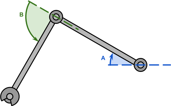
The solution that is proposing in this new series will only work on robotic arms with two joints. In the academic literature is often said that these robotic arms have two degrees of freedom. The reason for this will be very clear by looking at the diagram below. A robotic arm with two degrees of freedom can be modelled as a triangle, which is one of the most studied geometrical figures in geometry.
Let’s start by formalising the problem a little bit more. The two joints,  and
and  (both in black), can be rotated by (in blue) and (in green) degrees, respectively. This cause the end effector to move to a position
  .
.
Internal Angles
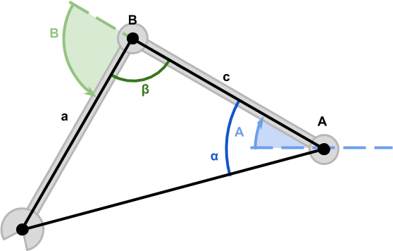
We can use the three points , and to construct a triangle with internal angles  ,
,  and
and  , like the one below.
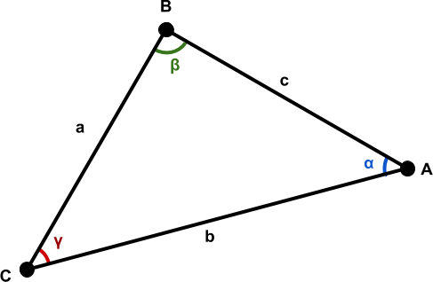
While these three angles are unknown, we know the length of all edges.
- The segment
 represents the arm and has length
  ;
; - The segment
 represents the forearm and has length
  ;
; - The segment
 represents the distance between the shoulder joint and the hand, and has length
  .
.
Knowing the three sides of a triangle is enough to find all of its angles. This is possible thanks to the law of cosines, a generalisation of Pythagora’s theorem for triangles that are not necessarily at right angles.
The two angles that are needed to control the robotic arm are and . Let’s start with , which can be calculated using the law of cosines on :
(1) 
We can refector (1) to extract  :
:
![\[ \begin{split} \cos{\alpha} & =\frac{a^2-b^2-c^2}{-2bc} = \\ & =\boxed{\frac{b^2+c^2-a^2}{2bc}} \end{split} \]](https://www.alanzucconi.com/wp-content/ql-cache/quicklatex.com-c03cc872bd0b62bcf17cb96446d08e3f_l3.png "Rendered by QuickLaTeX.com")
What is now needed is to use the inverse cosine function  (also known as arcosine) to find the :
(2) 
With the same procedure, we can apply the law of cosine once again to find :
![\[b^2 = a^2 + c^2 - 2ac \cos{\beta}\]](https://www.alanzucconi.com/wp-content/ql-cache/quicklatex.com-2eaf92ed4e4609c122fb29644f32721e_l3.png "Rendered by QuickLaTeX.com")
![\[\cos{\beta}=\frac{a^2 + c^2 -b^2}{2ac}\]](https://www.alanzucconi.com/wp-content/ql-cache/quicklatex.com-0a347b2694deacd8027582849e059034_l3.png "Rendered by QuickLaTeX.com")
(3) 
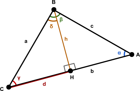
The segment  divides the triangle
  into two right triangles:
  and
and  . This proof is a natural consequence of applying Pythagora’s theorem to both triangles:
(4) 
(5) 
Both (4) and (5) are now expressed in terms of  . We can equate them to obtain:
![\[ \begin{split} \boxed{a^2 -d^2} & = \boxed{c^2 - \left(b-d\right)^2} \\ a^2 - d^2 &= c^2 - \left(b^2 + d^2 - 2 bd\right) \\ a^2 - d^2 & = c^2 - b^2 - d^2 + 2 bd \\ a^2 \xcancel{- d^2} & = c^2 - b^2 \xcancel{- d^2} + 2 bd\\ a^2 & = c^2 - b^2 + 2 bd \\ \end{split} \]](https://www.alanzucconi.com/wp-content/ql-cache/quicklatex.com-1e490ca3ead10db6c5901b4af4e60ad4_l3.png "Rendered by QuickLaTeX.com")
which can be rearrenged as:
(6) 
Equation (6) is how the Law of cosines was transcribed in Euclid’s Proposition 12 from Book 2 of the Elements.
To get to the modern form of the equation, we need to apply some trigonometry. Since (5) is a right triangle, we can express the segment  as:
as:
(7) 
where  can be found by remembering that the angles of a triangle sums up to
  (or, equivalently,
  radians):
(8) 
Substituting into (7) we obtain:
(9) 
The last step is a consequence of the well-known co-function identity which states that:
![\[ \sin\left(\frac{\pi}{2} - \gamma\right) = \cos{\gamma} \]](https://www.alanzucconi.com/wp-content/ql-cache/quicklatex.com-3f3f96e222dcf778ae425251c4f45ad3_l3.png "Rendered by QuickLaTeX.com")
We can now use (9) to replace in (6), which gives us the modern form of the law of cosines:
(10) 
Joint Angles
Using the law of cosines we have calculated the values for and , which are the internal angles of the triangle created by the robotic arm. However, the angles we really need are (in blue) and (in green).
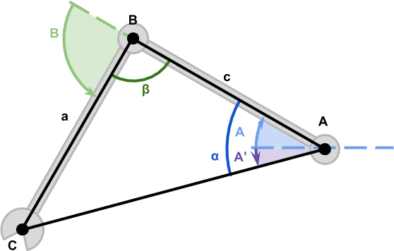
Let’s start by calculating , which is easier. It is obvious from the diagram above that and sum up to (equal to radians). This means that:
(11) 
Calculating is not much different. The only different here is that we need to take into account  (in purple), which is the angle of the segment
  . This can be calculated using the arcotangent function
  :
:
(12) 
Which leads to:
(13) 
The sign of the angles , and is mostly arbitrary and depends on the way each joint move.
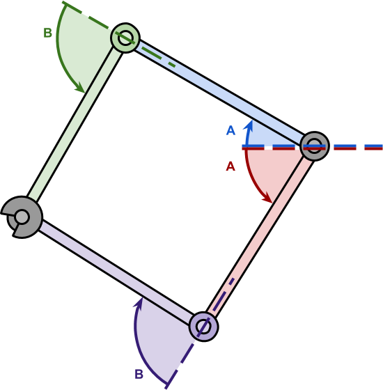
While the angles and are indeed different, the derivation remains essentially the same with the only exception of (13) and (11).
What’s Next…
This post concludes the introduction on the Mathematics of Inverse Kinematics for robotic arms with two degrees of freedom.
The next post will explore how we can use the equations derived to efficiently move a robotic arm in Unity.
You can read the rest of this online course here:
A follow-up that focuses on 3D is also available:
- Part 3. Inverse Kinematics in 3D
The line art animals that have been featured in this tutorial have been inspired by the work of WithOneLine.
Download
Become a Patron!
You can download all the assets used in this tutorial to have a fully functional robotic arm for Unity.
| Feature | Standard | Premium |
| Inverse Kinematics | ✅ | ✅ |
| Multiple Solutions | ❌ | ✅ |
| Smooth Reaching | ❌ | ✅ |
| Test Scene | ❌ | ✅ |
| Test Animations | ❌ | ✅ |
| Download | Standard | Premium |
💖 Support this blog
This website exists thanks to the contribution of patrons on Patreon. If you think these posts have either helped or inspired you, please consider supporting this blog.
📧 Stay updated
You will be notified when a new tutorial is released!
📝 Licensing
You are free to use, adapt and build upon this tutorial for your own projects (even commercially) as long as you credit me.
You are not allowed to redistribute the content of this tutorial on other platforms, especially the parts that are only available on Patreon.
If the knowledge you have gained had a significant impact on your project, a mention in the credit would be very appreciated. ❤️🧔🏻
“the law of cosines, a generalisation of Pythagora’s theorem for triangles that are not necessarily right.” should read “not necessarily *at right angles*.”
Thank you!
Help!
At calculation 12 you introduce 4 new terms (Ax, Ay, Cx, Cy) with no explanation.
What are they?
Hi!
Both A and C are points, and so they both have X and Y coordinates.
A = (Ax, Ay), and C = (Cx, Cy).
I hope this makes it clear!
hello, I have a question. At the start you mention “The segment \overline{CA} represents the distance between the shoulder joint and the hand, and has length b.
Knowing the three sides of a triangle is enough to find all of its angles”
How do you know the length of b?
Because both A (start point) and C (end point) are known, b is simply the distance between them!
While that may vary, a and c do not, since the segments of the robotic arm are rigid!
Hello, I have a question. What software did you use to create these nice geometry diagrams?
Hi! I made them with Google Drawings!
Hello! I have a background mainly in art and animation and wanted to know where I could find more information on “procedural animation”? It seems like there is very little documentation on how this is done and this is one of maybe 3 in depth documents I can find on the concept. I don’t have a huge coding background and wanted to know if you would have any recommendations on where to start learning more about this from someone who seems to know what they are talking about? thanks!
Hi!
Not sure if you have seen it, but I have a much more gentle introduction to the topic!
I hope it helps!
https://www.alanzucconi.com/2017/04/17/procedural-animations/
Hi, I dont understand why A = α + A’
Look at the diagram below “Joint angles”.
It shows You can literally see that α = A – A’.
(A’ is negative, so it is subtracted to get the positive angle).
So: A = α + A’
if only the shoulder point and hand point are known, how are you getting the elbow?
That would be the point “B” in the diagrams. You can find it by rotating the segment “c” around “A” by “alpha” degrees!