Inverse Kinematics in 3D

This tutorial will teach you how to master inverse kinematics in 3D: the technique that solves the problem of moving a robotic arm to reach for a specific target.

You can read the rest of this online course here:

Part 1. Inverse Kinematics in 2D: The Mathematics
Part 2. Inverse Kinematics in 2D: The Code

A link to download the entire Unity package can be found at the end of this tutorial.

Introduction

There are a few topics that keep recurring on this blog: one of them is, without any doubt, inverse kinematics. I have tackled this fascinating problem in two series so far, for a total of 8 separate articles. And yet, there is still so much more to write about inverse kinematics in the context of video games.

What makes inverse kinematics so interesting and complex to require this many posts? The truth is that inverse kinematics is a problem that recurs not only in video games, but in both engineering and science in general. From the design of robotic arms to the understanding of motor control in the human brain, inverse kinematics—in one form or another—plays an important role.

A Brief Summary

The first series dedicated to the topic, An Introduction to Procedural Animations, came out in 2017 and further popularized the term “procedural animations” among indie developers. It provided a general solution based on a gradient descent algorithm, which could potentially be used on rather “exotic” riggings, such as tentacles and spider legs.

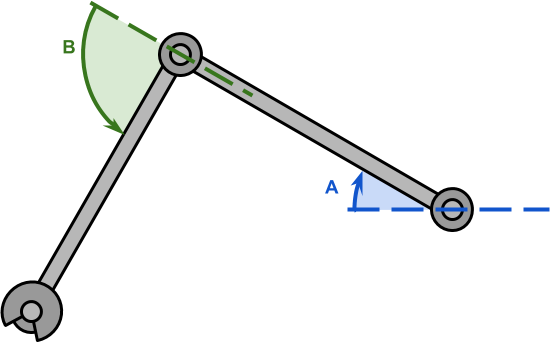
The second series, Inverse Kinematics in 2D, came out one year later and focused on a very specific case: a two-joint arm constrained in a 2D plane (below). Exactly as the name suggested: inverse kinematics in 2D. Each one of the two joints is controlled by an angle, $A$ and $B$ . By modulating these two angles, the tip of the robotic arm, called the end effector, will reach different locations.

The problem of inverse kinematics is to find the angles $A$ and $B$ so that the end effector reaches a desired target point. The animation below shows a robotic arm that is drawing a circle, aligned on the XY plane.

Technically speaking, the solution presented on Inverse Kinematics for Robotic Arms can work with potentially any number of joints. So why focusing on a less powerful technique? The answer is simple: efficiency. What made this worth writing about was the fact that, in the specific scenario just described, a solution can be found using a simple equation instead of a rather complex algorithm. That is thanks to the fact that we can imagine the robotic arm as a triangle (below) with two internal angles $\alpha$ and $\beta$ .

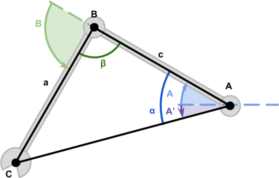
With a little bit of trigonometry, we found out the values for such angles to be:

(1) $\begin{equation*} \alpha = \cos^{-1}{\left(\frac{b^2+c^2-a^2}{2bc}\right)} \end{equation*}$

(2) $\begin{equation*} \beta=\cos^{-1}{\left(\frac{a^2 + c^2 -b^2}{2ac}\right)} \end{equation*}$

where $a$ , $b$ and $c$ are the sides of this “imaginary” triangle that we constructed.

However, the joints of the robotic arm are controlled using $A$ and $B$ , which turns out to be:

(3) $\begin{equation*} A = \alpha + A' \end{equation*}$

(4) $\begin{equation*} B = \pi - \beta \end{equation*}$

where:

(5) $\begin{equation*} A' = \tan^{-1}{\left(\frac{C_Y-A_Y}{C_X-A_X}\right)} \end{equation*}$

📚 Show me the derivation!

The full derivation can be found in the article titled Inverse Kinematics in 2D: The Mathematics.

Extending into the Third Dimension

If you have followed the Inverse Kinematics in 2D series before, there should not be anything new in the previous section. If you have not, do not worry: that is all you need to know.

What makes that simplified case worth discussing, is that it can be used as the starting point for solving inverse kinematics in 3D.

First of all, we need to understand that the scenario of a two-joint arm in 2D is a problem with two degrees of freedom (2DOF). Conversely to what one might imagine, it does not mean that we have two segments; but that we have control over two variables (which, in this case, turns out of to be the joint angles).

When we extend this problem to the third dimension, our robotic arm still has two segments and two joints. However, the problem has now three degrees of freedom (3DOF), if we assume that we can also rotate the arm freely around its first joint.

Under this new scenario, the second joint ( $B$ ) remains unchanged. However, we assume that the first one ( $A$ ) can now freely rotate in another dimension. Because of this, the first joint is often referred to as the hip, and the second as the knee. Your knee has generally only one degree of freedom (forwards/backwards), while your hip has two (forwards/backwards and inwards/outwards). The angle around which the hips rotates is indicated with $\theta$ .

We can imagine a robotic arm in which both joints can have two degrees of freedom, for a total of four. The problem at that point is that there will be multiple solutions, making our approach not effective anymore. “Leg-like” robotic arms (meaning: arms that have a hip and a knee joints) are very common both in games and in the industry in general. So this approach is probably worth studying.

If you have read the previous articles, you might remember that if the target is reachable in 2D, there are always two “specular” solutions (below).

The same problem occurs in 3D; this time, the solutions are infinite. This is because the configuration can rotate around the axis of symmetry represented by the straight line that connects the origin from the target. The solution is to… focus on just one solution! In this tutorial, we will focus on the most simple to find, which assumes (0, 1, 0) as the “up” direction.

From 2D to 3D

So far, we only know how to solve the problem of inverse kinematics when the movement is constraints to the XY plane. The trick to go from 2D to 3D is to re-use the 2D solution. The animation below shows a robotic arm reaching for a point in 3D space, which revolves around the Y-axis. It is pretty obvious to see that the only thing the arm does is to revolve as well; its angles $A$ and $B$ are not changing, only $\theta$ does.

This means that, if we know how to perform IK on the XY plane (and we do!) we know how to perform it on the entire XYZ space with two simple rotations. Conceptually, we can solve the problem in three steps:

Rotate the target point around the Y-axis, until it lies on the XY plane
Move the robotic arms so that it can reach for the point, as if it was in 2D
“Undo” the rotation by rotating the entire robotic arm in the opposite direction on the Y-axis.

We can do this more efficiently by simply performing the 2D inverse kinematics not on the XY plane, but on the vertical plane passing from the root of the robotic arm to the target point.

Rotation Around Y-Axis

To perform inverse kinematics in 3D, the first thing that we need to calculate is $\theta$ , which is the angle around which the entire robotic arm revolves. This is the extra degree of freedom added to the hip joint.

The best way to find it, is to assume that the robotic arm has already reached the position (meaning that $C$ is already at the target position) and calculating the resulting angle $\theta$ . Since $\theta$ is the angle made by the hip around the Y-axis, we can look at the robotic arm straight from the top. With a top-down view over the XZ plane (below), the robotic arm looks like a straight line. This is because, exception made for the hip, the other two joints are constraints on a plane.

If we look at the segment $\overline{AC}$ as the hypothenuse of a right triangle, we can use a bit of trigonometry to calculate the angle $\theta$ :

(6) $\begin{equation*} \theta = \tan^{-1}{\left(\frac{\Delta z}{\Delta x}\right)} = \tan^{-1}{\left(\frac{C_Z-C_Z}{C_X-A_X}\right)} \end{equation*}$

📚 Show me the derivation!

Calculating the angle between two points is a pretty common problem for game developers, which can be solved easily with a bit of trigonometry.

The trick, in this case, is to introduce the slope of a line (below), which is the ratio between its rise ( $\Delta y$ ) and run ( $\Delta x$ ). The slope of a line can be calculated between any two given, distinct points, and it yields the same result.

The slope of a line has a direct relationship with the angle of the line $\gamam$ :

(7) $\begin{equation*} \frac{\Delta y}{\Delta x} = \tan{\gamma} \end{equation*}$

If you have studied trigonometry, you should in fact recognise that the rise $\Delta y$ is in fact $\sin{\gamma}$ and the run $\Delta x$ is $\cos{\gamma}$ . And the tangent function is, by definition, the ration between sine and cosine.

To extract $\gamma$ from (7) we can use the inverse tangent function, which is known as arctangent:

(8) $\begin{equation*} \gamma = \tan^{-1}{\left(\frac{\Delta y}{\Delta x}\right)} \end{equation*}$

While this works really nice in theory, there are a few issues with the sign of $\Delta x$ and $\Delta y$ . The slope, in fact, yields the same result when $\Delta x$ and $\Delta y$ are both positive or both negative. But, from a geometrical point of view, those correspond to two opposite angles! The solution is to not use $\tan^{-1}$ directly, but its “programming” cousin, atan2. Most frameworks have an implementation of the arctangent function that takes two parameters, usually called dy and dx.

⭐ Suggested Unity Assets ⭐

Unity is free, but you can upgrade to Unity Pro or Unity Plus subscriptions plans to get more functionality and training resources to power up your projects.

Inverse Kinematics on the WY Plane

Technically speaking, knowing $\theta$ is more than enough to solve inverse kinematics in 3D. What we could do, in fact, is to follow the algorithm presented in the previous section: rotating the target point by $-\theta$ degrees around the Y axis, performing the inverse kinematics on the XY plane, and finally rotating the entire arm by $+\theta$ degrees.

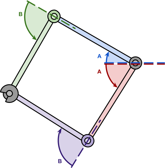
A quicker version is to perform the inverse kinematics not on the 2D plane, but directly on the vertical plane passing through the hip joint and the target point. There is, unfortunately, something that is preventing us from doing so. Let’s look once again at the diagram which indicates all of the angles used:

In order to calculate $A$ , which is the angle that controls the first joint, we need to calculate $A'$ . That is the angle between the first joint and the target point, If we recall equation (5) used to calculate $A'$ , we notice one big problem: it assumes all points lie on the XY plane:

$\begin{equation*} A' = \tan^{-1}{\left(\frac{C_Y-A_Y}{C_X-A_X}\right)} \end{equation}$

In our 3D scenario, unfortunately the robotic arm would be rotated by $\theta$ degrees around the Y-axis. The new diagram stays mostly the same, however, if we rotate our view together with the robotic arm. We call this new reference frame WY, since the X-axis is now replaced by W, which was the X-axis, not rotated by $\theta$ degrees around the Y-axis.

We cannot simply do $D_X-A_X$ as we did for $\Delta y$ . This is because while $C$ and $D$ are aligned on the Y-axis, $A$ and $D$ are not aligned to the X-axis. They are aligned to the W-axis. The best way to calculate $\Delta w$ is, consequently, to get the distance from $A$ to $D$ . This loses the sign of $\Delta w$ , but it luckily bears no real issue on our calculations. If your arm happens to move in the opposite direction, simply flip the sign of $\Delta w$ in your code.

(9) $\begin{equation*} A' = \tan^{-1}{\left(\frac{\Delta y}{\Delta w}\right)} =\tan^{-1}{\left(\frac{C_Y-D_Y}{\left|\overline{A D}\right|}\right)} \end{equation*}$

where $\left|\overline{A D}\right|$ is the length of the segment from $A$ to $D$ . It can be calculated easily with a function such as Vector3.Distance, or you could also use Pythagoras’ theorem directly:

(10) $\begin{equation*} \begin{align} A' &=& \tan^{-1}{\left(\frac{C_Y-D_Y}{ \sqrt{\left(C_X - A_X\right)^2+\left(A_Y- A_Y\right)^2+\left(C_Z - A_Z\right)^2 }\right)}} = \\ &=& \tan^{-1}{\left(\frac{C_Y-D_Y}{ \sqrt{\left(C_X - A_X\right)^2+\left(C_Z - A_Z\right)^2 }\right)}} \end{align} \end{equation*}$

In the equation above, the Y contribution from the Pythagoras’ theorem cancels itself out because the point $D$ has the same Y component of $A$ , so their $\Delta y$ is zero.

Now, we really do have everything to perform inverse kinematics in 3D for robotic arms with one keen and hip joint:

(11) $\begin{equation*} \theta = \tan^{-1}{\left(\frac{C_Z-C_Z}{C_X-A_X}\right)} \end{equation*}$

(12) $\begin{equation*} A = \cos^{-1}{\left(\frac{b^2+c^2-a^2}{2bc}\right)} + \tan^{-1} { \left( \frac {C_Y-D_Y} { \sqrt { \left(C_X - A_X\right)^2 +\left(C_Z - A_Z\right)^2 } } \right)} \end{equation*}$

(13) $\begin{equation*} B &=& \pi - \cos^{-1}{\left(\frac{a^2 + c^2 -b^2}{2ac}\right)} \end{equation*}$

While looking scary, these equations are simple to implement and allows to perfom inverse kinematics in 3D as fast as possible.

What’s Next…

The next tutorial in this series will show how to use inverse kinematics to create believable legged creatures. Yes, the anticipated tutorial about inverse kinematics for spider legs is finally coming!!!

Unity Package Download

Become a Patron!
You can download all the assets used in this tutorial to have a fully functional robotic arm for Unity.

Feature	Standard	Premium
Inverse Kinematics in 3D	✅	✅
Multiple Solutions	❌	✅
Smooth Reaching	❌	✅
Test Scene	❌	✅
Test Animations	❌	✅
Download	Standard	Premium

Additional Resources

💖 Support this blog

This website exists thanks to the contribution of patrons on Patreon. If you think these posts have either helped or inspired you, please consider supporting this blog.

Follow @AlanZucconi

📧 Stay updated

You will be notified when a new tutorial is released!

📝 Licensing

You are free to use, adapt and build upon this tutorial for your own projects (even commercially) as long as you credit me.

You are not allowed to redistribute the content of this tutorial on other platforms, especially the parts that are only available on Patreon.

If the knowledge you have gained had a significant impact on your project, a mention in the credit would be very appreciated. ❤️🧔🏻

Tony Nguyen

October 8, 2020

Hi, Great Article first of all! The implementation is really nice and simple. I just have one problem that I can’t solve, how would you go with adding an Pole Target to the ik?

Reply to Tony
Andrei

October 28, 2020

in the 6th equation shouldn’t it be Cz-Az?

Reply to Andrei
- Andrei
  
  October 28, 2020
  
  also, why in th10 equation we have Ay-Ay?
  
  Reply to Andrei
Ryan Weiss

April 2, 2023

Hello. Did you ever release any article or sample on animating the spider legs, or is it in the Premium package? ;-p

Reply to Ryan

Webmentions

Inverse Kinematics in 2D - Part 1 - Alan Zucconi April 2, 2023

[…] Part 3. Inverse Kinematics in 3D […]

Inverse Kinematics in 2D - Part 2 - Alan Zucconi April 2, 2023

Published

September 14, 2020

Alan Zucconi in C#, Maths, Programming, Tutorial, Unity | September 14, 2020