
This is the second part of the tutorial on volumetric atmospheric scattering. In this post we will start deriving the equations that govern this complex, yet beautiful optical phenomenon.
You can find all the post in this series here:
- Part 1. Volumetric Atmospheric Scattering
- Part 2. The Theory Behind Atmospheric Scattering
- Part 3. The Mathematics of Rayleigh Scattering
- Part 4. A Journey Through the Atmosphere
- Part 5. A Shader for the Atmospheric Sphere
- Part 6. Intersecting The Atmosphere
- Part 7. Atmospheric Scattering Shader
- 🔒 Part 8. An Introduction to Mie Theory
You can download the Unity package for this tutorial at the bottom of the page.
Introduction
In the first part of this tutorial, we have discussed how light can be deflected by the air molecules present in a planet’s atmosphere. This process is called scattering, and we have highlighted two special cases. Out-scattering occurs when a ray of light that was directed towards the camera is deflected away from it (diagram below).
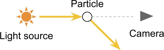
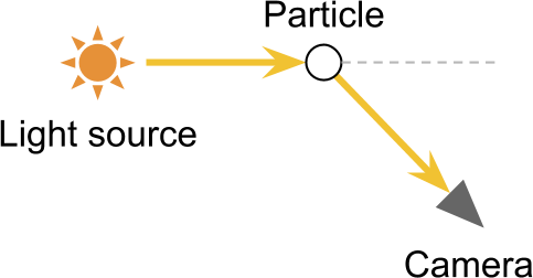
Conversely, in-scattering occurs when a ray of light is deflected directly towards the camera.
The Transmittance Function
To calculate the amount of light transmitted to the camera, is helpful to take the same journey that light rays from the sun undergo. By looking at the diagram below, is easy to see that light rays reaching  travel through empty space. Since nothing is in their path, all the light reaches without being subjected to any scattering effect. Let’s indicate with
  the amount of unscattered light that the point receives from the sun. During its journey to
  , light enters the planet’s atmosphere. Some rays will collide with the molecules suspended in the air, bouncing in different directions. The result is that some of the light is scattered away from the path. The amount of light reaching (denoted with
  ) will be lower than .
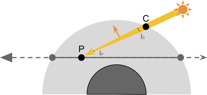
The ratio between and is called transmittance:
![\[T\left(\overline{CP}\right) = \frac{I_P}{I_C}\]](https://www.alanzucconi.com/wp-content/ql-cache/quicklatex.com-8471db80c74dc57d8fb698e7d94374c7_l3.png "Rendered by QuickLaTeX.com")
and we can use it to indicate the percentage of light that is not scattered (transmitted) during the journey from to . We will explore later the nature of this function. For now, the only thing you need to know is that it corresponds to the contribution of atmospheric out-scattering.
Consequently, the amount of light that receives is:
![\[I_P = I_C \, T\left(\overline{CP}\right)\]](https://www.alanzucconi.com/wp-content/ql-cache/quicklatex.com-2d3a9843d045fd5a8a087c5235ed90bd_l3.png "Rendered by QuickLaTeX.com")
The Scattering Function
The point receives light directly from the sun. However, not all that light passing through is transferred back to the camera. To calculate how much light actually reaches the camera, we need to introduce yet another concept: the scattering function  . Its purpose is to indicate how much light is deflected in a certain direction. If we look at the diagram below, we notice that only those rays of lights that are deflected by an angle of
  are going to be directed towards the camera.
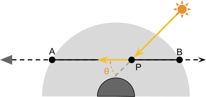
The value of  indicates the ratio of light deflected by radians. This function is at the heart of our problem, and we will explore its nature in a future post. For now, the only thing you have to know is that it depends on the colour of the incoming light (indicated by its wavelength
  ), the scattering angle and the altitude
  of . The reason why the altitude is important is because the atmospheric density changes as a function of the altitude. And the density is, ultimately, one of the factors to determine how much light is scattered.
We now have all the tools necessary to write a general equation that shows how much light is transferred from to  :
:
![\[I_{PA} = \boxed{I_P} \, S\left(\lambda,\theta,h\right) \, T\left(\overline{PA}\right)\]](https://www.alanzucconi.com/wp-content/ql-cache/quicklatex.com-8a16120274a4f00e03931e5d8eb65b24_l3.png "Rendered by QuickLaTeX.com")
We can expand using the previous definition:
![\[I_{PA} = \boxed{I_C \, T\left(\overline{CP}\right)}\, S\left(\lambda,\theta,h\right) \,T\left(\overline{PA}\right)=\]](https://www.alanzucconi.com/wp-content/ql-cache/quicklatex.com-17226a9b7674789f3f2c4a197a9572db_l3.png "Rendered by QuickLaTeX.com")
![\[= \underset{\text{in-scattering}}{ \underbrace{I_C \,S\left(\lambda,\theta,h\right)} }\, \underset{\text{out-scattering}}{\underbrace{T\left(\overline{CP}\right)\, T\left(\overline{PA}\right)}}\]](https://www.alanzucconi.com/wp-content/ql-cache/quicklatex.com-f99a8bddf602fd8372af3c89a8939a03_l3.png "Rendered by QuickLaTeX.com")
The equation should be self explanatory:
- Light is travels from the sun to , unscattered in the vacuum of space;
- Light enters the atmosphere and travels from to . In doing so, only the fraction
 reaches its destination due to out-scattering;
 - Part of the light that has reached from the sun is deflected back to the camera. The ratio of light subjected to in-scattering is
 ;
; - The remaining light travels from to , and once again only the fraction
 is transmitted.
The Numerical Integration
If you have paid attention to the previous paragraphs, you might have noticed an apparent inconsistency in the way intensity have been written. The symbol  indicates the amount of light transferred from to . However, that quantity does not account for all the light that receives. In this simplified models of atmospheric scattering, we are taking into account the in-scattering from every point along the camera’s line of sight through the atmosphere.
The total amount of light receives,  , is calculated by adding together the contribution from all the points
  . Mathematically speaking, there are infinitely many points in the segment
  , so looping through all of them will be impossible. What we can do, however, is splitting into many smaller segments of length
  (diagram below), and accumulating the contribution of each.
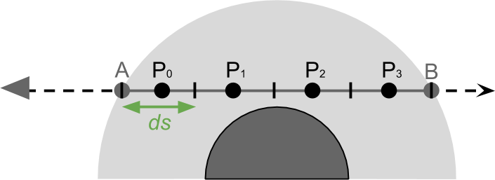
This process of approximation is called numerical integration, and leads to the following expression:
![\[I_A = \sum_{P \in \overline{AB}} {I_{PA}\, ds }\]](https://www.alanzucconi.com/wp-content/ql-cache/quicklatex.com-73cd82418fd97766d94d6358af98d6a3_l3.png "Rendered by QuickLaTeX.com")
The more points we’ll take into account, the more accurate our final result will be. In reality, what we will have to do in our atmospheric shader is to loop through several points  inside the atmosphere, accumulating their contribution to the overall result.
, we are weighing their contributions according to their length. The more points we have, the less important each one of them is.
An alternative way to look at this is that multiplying by “averages out” the contribution of all the points.
Directional Light
If the sun is relatively close, it is best modelled as a point light source. In that case, the amount of light received at depends on the distance from the sun itself. If we are talking about planets, however, we can often assume the sun to be so distant that its rays arrive at the planet all with the same angle. If that’s the case, we can model the sun as a directional light source. The light received from directional light sources remain constant regardless of the distance it travels. Hence, every point receives the same amount of light, and the direction towards the sun is the same for all points.
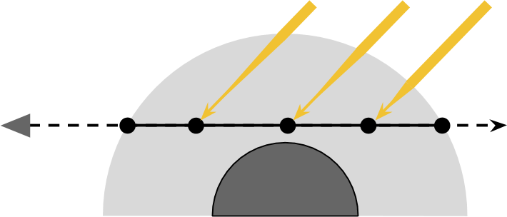
We can use this assumption to simplify our set of equations.
Let’s replace with the constant  , which represents the sun intensity.
![\[I_A = \sum_{P \in \overline{AB}} {\boxed{I_{PA}}\, ds } =\]](https://www.alanzucconi.com/wp-content/ql-cache/quicklatex.com-8f734e88963dd38415b3ffa2917e06b5_l3.png "Rendered by QuickLaTeX.com")
![\[= \sum_{P \in \overline{AB}} {\boxed{I_C \,S\left(\lambda,\theta,h\right) \,T\left(\overline{CP}\right)\, T\left(\overline{PA}\right)}\, ds }=\]](https://www.alanzucconi.com/wp-content/ql-cache/quicklatex.com-a45c71e9bd030da4e3e8d483ab4132ac_l3.png "Rendered by QuickLaTeX.com")
![\[= I_S \sum_{P \in \overline{AB}} {S\left(\lambda,\theta,h\right) \,T\left(\overline{CP}\right) \, T\left(\overline{PA}\right) \,ds }=\]](https://www.alanzucconi.com/wp-content/ql-cache/quicklatex.com-62e9e866263cc8d02c28a295104ad9f2_l3.png "Rendered by QuickLaTeX.com")
There is another optimisation that we can perform, and it involves the scattering function . If the sunlight always comes from the same direction, the angle becomes a constant. We will see in a future post how the directional contribution of can be factored out of the summation. For now, let’s keep it inside.
Absorption Coefficient
When describing the possible outcomes of the interaction between light and air molecules, we have only introduced two. Passing straight through, or being deflected. There is a third possibility. Some chemical compounds absorb light. The atmosphere on Earth has plenty of chemicals with such a property. Ozone, for instance, is present in the higher atmosphere and is known to react strongly to ultraviolet light. Its presence, however, has virtually no effect on the colour of the sky, since it absorbs light outside the visible spectrum.Here on Earth, the contribution of light-absorbing chemicals is often ignored.
Here on Earth, the contribution of light-absorbing chemicals is often ignored. The same cannot be done for other planets. The typical colouration of Neptune and Uranus, for instance, is caused by the abundant presence of methane in their atmospheres. Methane is known for absorbing red light, resulting in a blue hue. In the rest of this tutorial we will ignore the absorption coefficient, although we will add a way to tint the atmosphere.
❓ What causes the Sun to turn red during the Ophelia storm of 2017?If we look at the colours of the visible spectrum (below), it’s easy to see that the if enough blue light is scattered, the sky can indeed turn yellow or red.

One might be tempted to say that the colour of colouration of the sky is related to the tint from the yellow Saharan sand. However, the same effect can be seen during large fires due to smoke particles, which tend to be black.
Coming Next…
In this tutorial, we have derived a very general form of the equations that govern single scattering. The approach described is, in theory, applicable to all translucent volumes receiving light from a single source.
The two key aspects are, of course, the transmittance function  and the scattering function . In the next tutorial, we will explore their nature, and derive equations depending on the physical properties of a planet’s atmosphere.
You can find all the post in this series here:
- Part 1. Volumetric Atmospheric Scattering
- Part 2. The Theory Behind Atmospheric Scattering
- Part 3. The Mathematics of Rayleigh Scattering
- Part 4. A Journey Through the Atmosphere
- Part 5. A Shader for the Atmospheric Sphere
- Part 6. Intersecting The Atmosphere
- Part 7. Atmospheric Scattering Shader
- 🔒 Part 8. An Introduction to Mie Theory
Download
Become a Patron!
You can download all the assets necessary to reproduce the volumetric atmospheric scattering presented in this tutorial.
| Feature | Standard | Premium |
| Volumetric Shader | ✅ | ✅ |
| Clouds Support | ❌ | ✅ |
| Day & Night Cycle | ❌ | ✅ |
| Earth 8K | ✅ | ✅ |
| Mars 8K | ❌ | ✅ |
| Venus 8K | ❌ | ✅ |
| Neptune 2K | ❌ | ✅ |
| Postprocessing | ❌ | ✅ |
| Download | Standard | Premium |
💖 Support this blog
This website exists thanks to the contribution of patrons on Patreon. If you think these posts have either helped or inspired you, please consider supporting this blog.
📧 Stay updated
You will be notified when a new tutorial is released!
📝 Licensing
You are free to use, adapt and build upon this tutorial for your own projects (even commercially) as long as you credit me.
You are not allowed to redistribute the content of this tutorial on other platforms, especially the parts that are only available on Patreon.
If the knowledge you have gained had a significant impact on your project, a mention in the credit would be very appreciated. ❤️🧔🏻
Thank you very much! I learn a lot from this.
I’m glad it helped!