
You can read all the posts in this series here:
- Part 1. An Introduction to DeepFakes and Face-Swap Technology
- Part 2. The Ethics of Deepfakes
- Part 3. How To Install FakeApp
- Part 4. A Practical Tutorial for FakeApp
- Part 5. An Introduction to Neural Networks and Autoencoders
- Part 6. Understanding the Technology Behind DeepFakes
- Part 7. How To Create The Perfect DeepFakes
An Introduction to Neural Networks
To understand how deepfakes are created, we first have to understand the technology that makes them possible. The term deep comes from deep learning, a branch of Machine Learning that focuses on deep neural networks. They have been covered extensively in the series Understanding Deep Dreams, where they were introduced to for a different (yet related) application.
Neural networks are computational system loosely inspired by the way in which the brain processes information. Special cells called neurons are connected to each other in a dense network (below), allowing information to be processed and transmitted.
In Computer Science, artificial neural networks are made out of thousands of nodes, connected in a specific fashion. Nodes are typically arranged in layers; the way in which they are connected determines the type of the network and, ultimately, its ability to perform a certain computational task over another one. A traditional neural network might look like this:
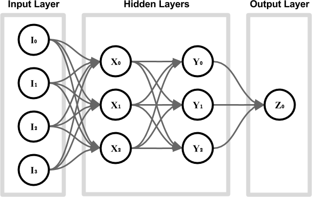
Each node (or artificial neuron) from the input layer contains a numerical value that encodes the input we want to feed to the network. If we are trying to predict the weather for tomorrow, the input nodes might contain the pressure, temperature, humidity and wind speed encoded as numbers in the range ![\left[-1,+1\right]](https://www.alanzucconi.com/wp-content/ql-cache/quicklatex.com-ae9ff7abb09a3e5a1f27ed8b3ef28b87_l3.png "Rendered by QuickLaTeX.com") . These values are broadcasted to the next layer; the interesting part is that each edge dampens or amplifies the values it transmits. Each node sums all the values it receives, and outputs a new one based on its own function. The result of the computation can be retrieved from the output layer; in this case, only one value is produced (for instance, the probability of rain).
. These values are broadcasted to the next layer; the interesting part is that each edge dampens or amplifies the values it transmits. Each node sums all the values it receives, and outputs a new one based on its own function. The result of the computation can be retrieved from the output layer; in this case, only one value is produced (for instance, the probability of rain).
When images are the input (or output) of a neural network, we typically have three input nodes for each pixel, initialised with the amount of red, green and blue it contains. The most effective architecture for image-based applications so far is convolutional neural network (CNN), and this is exactly what Deep Fakes is using.
Training a neural network means finding a set of weights for all edges, so that the output layer produces the desired result. One of the most used technique to achieve this is called backpropagation, and it works by re-adjusting the weights every time the network makes a mistake.
The basic idea behind face detection and image generation is that each layer will represent progressively core complex features. In the case of a face, for instance, the first layer might detect edges, the second face features, which the third layer is able to use to detect images (below):

In reality, what each layer responds to is far from being that simple. This is why Deep Dreams have been originally used as a mean to investigate how and what convolutional neural networks learn.
Autoencoders
Neural networks come in all shapes and sizes. And is exactly the shape and size that determine the performance of the network at solving a certain problem. An autoencoder is a special type of neural network whose objective is to match the input that was provided with. At a first glance, autoencoders might seem like nothing more than a toy example, as they do not appear to solve any real problem.
Let’s have a look at the network below, which features two fully connected hidden layers, with four neurons each.
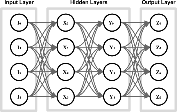
If we train this network as an autoencoder, we might encounter a serious problem. The edges that might converge to a solution where the input values are simply transported into their respective output nodes, as seen in the diagram below. When this happens, no real learning is happening; the network has rewired itself to simply connect the output nodes to the input ones.
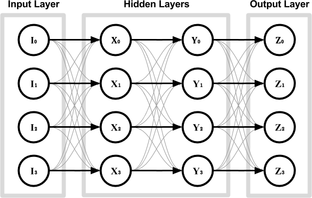
However, something interesting happens if one of the layers features fewer nodes (diagram below). In this case, the input values cannot be simply connected to their respective output nodes. In order to succeed at this task, the autoencoder has to somehow compress the information provided and to reconstruct it before presenting it as its final output.

If the training is successful, the autoencoder has learned how to represents the input values in a different, yet more compact form. The autoencoder can be decoupled into two separate networks: an encoder and a decoder, both sharing the layer in the middle. The values ![\left[Y_0, Y_1\right]](https://www.alanzucconi.com/wp-content/ql-cache/quicklatex.com-06a889d15ae5e8ee20bf6d9380fef993_l3.png "Rendered by QuickLaTeX.com") are often referred to as base vector, and they represent the input image in the so-called latent space.
are often referred to as base vector, and they represent the input image in the so-called latent space.
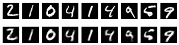
Autoencoders are naturally lossy, meaning that they will not be able to reconstruct the input image perfectly. This can be seen in the comparison below, taken from Building Autoencoders in Keras. The first row shows random images that have been fed, one by one, to a trained autoencoder. The row just below shows how they have been reconstructed by the network.
However, because the autoencoder is forced to reconstruct the input image as best as it can, it has to learn how to identify and to represents its most meaningful features. Because the smaller details are often ignored or lost, an autoencoder can be used to denoise images (as seen below). This works very well because the noise does not add any real information, hence the autoencoder is likely to ignore it over more important features.

Conclusion
The next post in this series will explain how autoencoders can be used to reconstruct faces.
You can read all the posts in this series here:
- Part 1. An Introduction to DeepFakes and Face-Swap Technology
- Part 2. The Ethics of Deepfakes
- Part 3. How To Install FakeApp
- Part 4. A Practical Tutorial for FakeApp
- Part 5. An Introduction to Neural Networks and Autoencoders
- Part 6. Understanding the Technology Behind DeepFakes
- Part 7. How To Create The Perfect DeepFakes
Leave a Reply