Unity 4D #3: Rendering 4D Objects

Follow @AlanZucconi

This article will explain how to render 4D objects in Unity, using three separate technique: orthographic projection, perspective projection and cross-section.

You can find all the articles in this series here:

• Part 1: Understanding the Fourth Dimension
• Part 2: Extending Unity from 3D to 4D
• Part 3: Rendering 4D Objects
• Part 4: Creating 4D Objects

A link to download the Unity4D package can be found at the end of this article.

Introduction

It is undeniable that what makes hyperdimensional objects so fascinating—and incidentally, so misunderstood—is their inherent mystery. A mystery that lies not so much in their own construction, but in our inability to grasp them with our imagination. As creatures that evolved in a 3D world, we are very ill-equipped to visualise 4D shapes in our heads. And something as intuitive as rotating a cube, can suddenly become incomprehensible when the very same rotation takes place in the fourth dimension.

While it is true that the real beauty of four-dimensional objects will forever be hidden in the hyperspace they belong to, it does not mean we have no effective ways to visualise them. After all, the monitor you are all reading from is effectively two-dimensional, but it is perfectly capable of visualising three-dimensional shapes. Playing a 3D game on a 2D monitor is not the same as being in that three-dimensional space, but is close enough for that illusion to work. The same principle applies to 4D objects: we cannot fully appreciate them, but we can still render them in a way that makes them understandable.

Map projections

The first issue is that there is not one “correct” way to bring a four-dimensional object into our three-dimensional realm. Instead, there are a variety of different techniques, each one with its own advantages and disadvantages. The exact same issue is not peculiar to hyperspace; it is an inherent, unavoidable problem that resurfaces every time we map something onto a different dimension. If you are familiar with geographical maps, you might also know that it is impossible to correctly project a 3D sphere onto a 2D surface. No matter how hard we try, we lose something. Geometrically speaking, we can say that a sphere is not isometric to a plane. Projecting a sphere onto a plane inevitably requires stretching and deforming its surface, in a way that distorts some of its properties.

And this is exactly why there are countless different ways to project Earth’s surface onto a map. While all attempts to capture the precision of Earth’s surface, they all care about preserving a different aspect of its complexity, at the expense of some other ones. The Mercator projection, for instance, is excellent at preserving local directions and shapes; while sacrificing relative sizes.

Wikipedia has a page (List of map projections, where the images above have been taken) that lists some of the most popular map projections; the article counts over 80 of them, and is far from being a comprehensive list.

This fact, alone, should help to understand that the issue of projecting higher-dimensional geometries onto lower ones is not unique to hyperspaces. It is something that plays an active role in our everyday lives, and that can have strong geographical, social and political repercussions. While rendering tesseracts in Unity is unlikely to have such an impact, it is important to remember that there is no right way of rendering 4D objects. There are many different ways, all imperfect, but each one trying to preserve an aspect of their very nature for us to appreciate.

Rendering 4D objects

The purpose of this article is to show the three most common ways in which 4D objects are usually rendered in Computer Graphics:

• Orthogonal Projection: one of the four components is dropped (usually ).
• Perspective Projection: the 4D shape casts a 3D shadow in our realm, similar to how a 3D shape casts a 2D shape.
• Cross-Section: only the part of the 4D shape that “intersects” our 3D realm is rendered.

The first two can be rendered using Unity’s LineRenderer component. If you are looking for something more professional, I would highly suggest Shapes by Freya Holmér.

Orthogonal Projection

In the field of Computer Graphics, 3D models are often rendered with a wiremesh connecting their vertices. Four-dimensional meshes can be stored—and rendered—in a similar way: through their vertices.

And the easiest way to visualise a set of 4D points in a 3D space, is to simply drop one of their coordinates. Incidentally, this is something that many 3D artists and designers are intimately familiar with: orthogonal projections. Several modern modelling software, from Maya to AutoCAD, offers the possibility of splitting the view into four separate windows, three of which are rendering the model without any perspective along the X, Y and Z axes.

Orthogonal projections are very valuable, as they offer a way to understand the shape of a complex object through four different perspectives at the same time. The animation below shows the orthographic projections of a 3D onto the X, Y and Z axes.

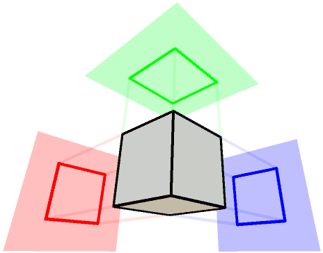
Projecting a cube onto the X axis effectively means rendering its wireframe after removing the X coordinate from each vertex. This results in a flat (i.e.: orthographic) projection which lies on the YZ plane.

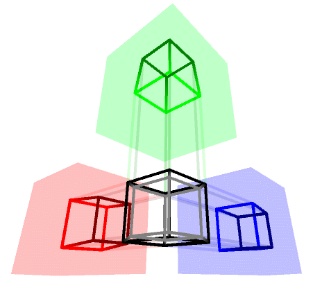
The orthographic projection of a 3D object produces three 2D images. The same principle applies to a 4D shape, which can be projected as four separate 3D objects.

The animation below shows the orthographic projection of a hypercube. The wireframe at the centre is rendering the XYZ components, while the other three are using WYZ (in red), XYZ (in green) and XYW (in blue).

The hypercube above is spinning simultaneously around its X, Y and Z, which is why its XYZ 3D projection doesn’t appear to change shape. The other 3D hyper-projections reveal how the part of the hypercube that lies beyond our realm actually rotates as well. And if you recall from the first article in the series, the projection of a rotating hypercube looks like a 3D cube being flipped inside-out.

The animation above is also using a “gentle” perspective projection, which will be explained in the next section. The colour of the wireframe also reflects how “deep” an edge is in hyperspace (black for , grey for ).

Perspective Projection

The main feature of orthographic projection is that objects look the same regardless of their distance from the camera. There are many scenarios in which this is highly desirable, for instance when modelling an object in a 3D software like AutoCAD or Maya. However, our brain infers distances also by relying on the fact that the further an object is, the smaller it gets. Orthographic projections do not add any distance-based distortions and this, paradoxically, impeaches our ability to sense depth.

When it comes to 4D shapes, their orthogonal projections can be quite crude, as edges often overlap and there is no sense of what is in front of what. To get around this, the wireframes of 4D meshes are often rendered using a perspective projection. This process is not dissimilar from how 3D objects cast 2D shadows.

There are several different approaches to translate this in four dimensions. One of the most common ones imagines a light placed at distance along the W axis, casting a 3D shadow of a 4D object. Assuming a generic vertex , the projected point can be calculated as:

(1)  

This is also akin to multiplying a 4D vector by the following perspective matrix:

(2)  

For a more visual explanation, I would suggest the following video:

Cross-section

There are countless ways to find the intersection between a 4D shape and a 3D space. But given the complexity of this task, it is easier to start a relaxed version of the problem. Relaxed problems are “simpler” questions that are easier to answer. When the relaxation is done properly, it makes it easier to answer complex questions incrementally.

In this section, we will see how to find the cross-section of a 4D object by first learning how to calculate the 3D intersection of its edges. And in order to do that, we will see how to determine if a 4D point is in our realm or not.

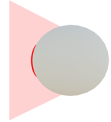
Intersection between a 4D point and a 3D space

How do we know when a 4D point manifests into our 3D space? Let’s start with something simpler: the equation of a line. There are many ways to define a line, resulting in equations that—despite all representing the same object—all look quite different. In 2D, you might be most familiar with the slope-intercept form:

(5)  

where is the slope (a measure of the line inclination) and is the y-intercept (where the line intersects the Y axis).

An equivalent variant of this equation is the normal form, which defines a line using a point and a normal vector orthogonal to the line. An arbitrary point belongs to the line if the following equation is satisfied:

(6)  

Here, the hat symbol is used to denote a unit vector, and the arrow symbol to denote a vector.

What makes the normal form, expressed with vectors, powerful, is that it works in any dimension. When the vectors have two elements, it denotes a line. When they have three elements, it denotes a plane. And when they have four dimensions, it denotes a space. It might not be immediately obvious to visualise this in 4D, but a hyperplane effectively divides the hyperspace in half, exactly like a line and a plane do on their respective dimensions. An arbitrary plane in 3D is defined by its centre point and normal vector; the same principle applies in 4D to identify a 3D space.

Generally speaking, 4D point belongs to the 3D space centered at and with normal when (6) is satisfied. For the center we can use and for the normal . In the same way the 3D normal of a 2D plane does not belong to the plane itself, the 4D normal of a 3D space does not belong to our realm.

Substituting the values in (6), we get the following expression:

(7)  

The result is fairly intuitive and is aligned with the general idea that a 4D point belongs to our 3D space if and only if its coordinate is equal to .

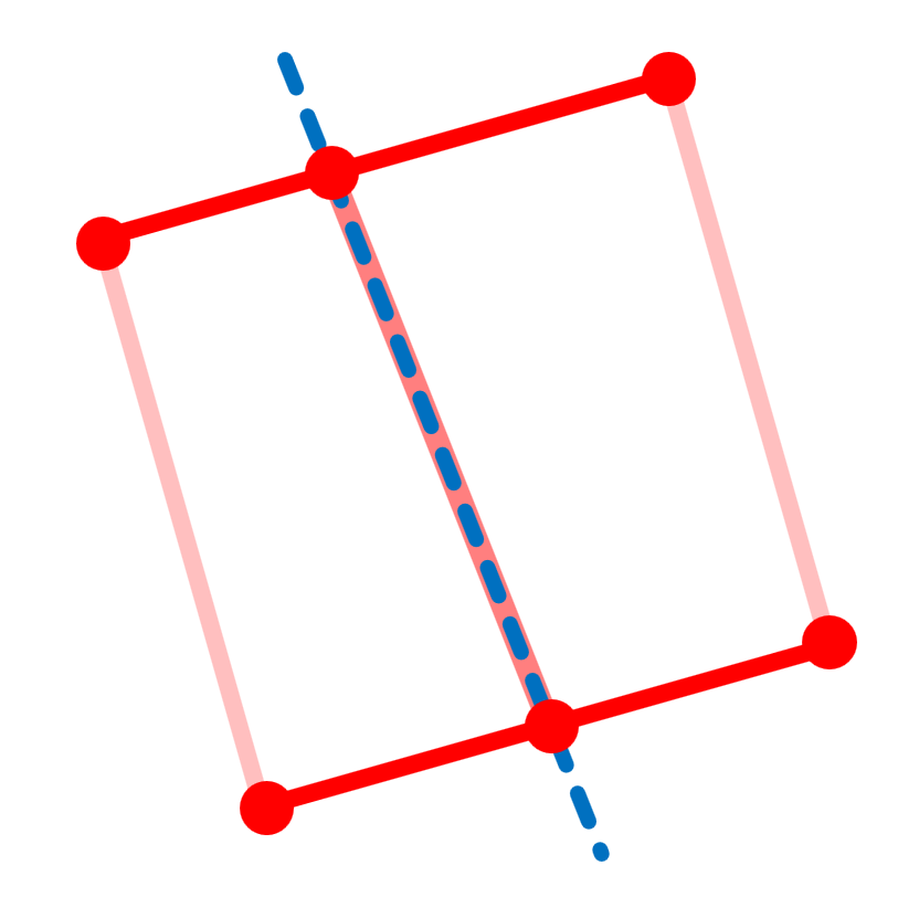
Intersections between a 4D segment and a 3D space

The previous section explained that a 4D point belongs to our realm if and only if its component is zero. We can use that information to solve a slightly more complex problem: the 3D intersections with a 4D segment.

Without the risk of any loss in generality, it helps to visualise what this means in two dimensions. A segment (in any dimension) is a straight line connecting two points, namely and . There are three solutions possible:

• No intersection: the segment never crosses the hyperplane.
• One intersection: the segment crosses the hyperplane, intersecting it at exactly one point.
• Infinite intersections: the segment lies on the hyperplane, so all of its points are intersecting it.

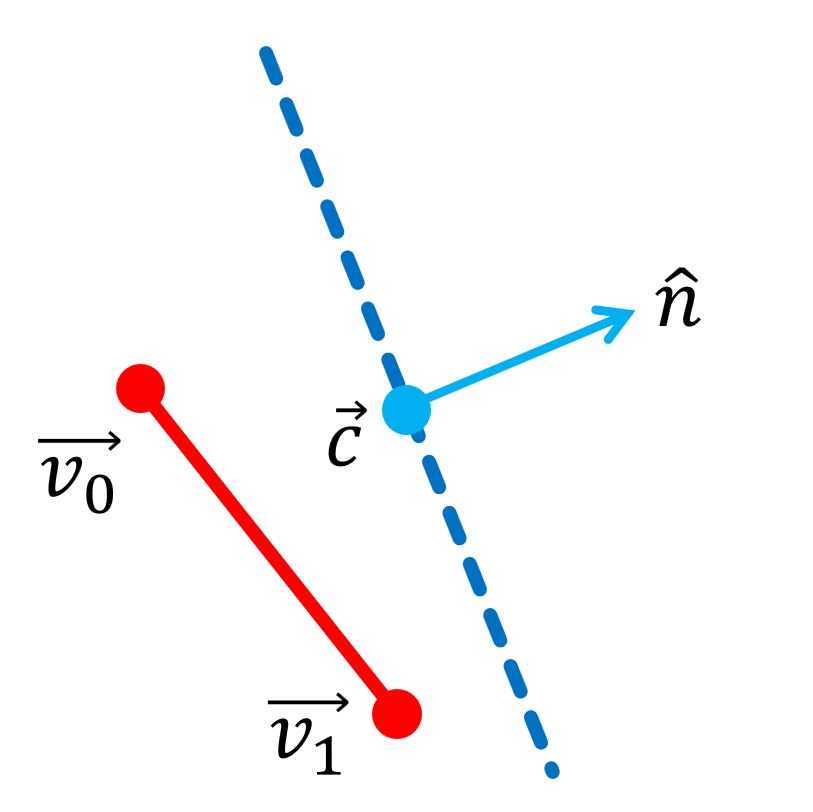
It is easy to see from the diagrams above that there is no scenario in which only a sub-segment lies on the hyperplane. This is an important factor to keep in mind, and we can prove it—at least intuitively—by understanding what happens along a line that connects to points. The only points from the segment that belongs to our realm are the ones which satisfy the property . To understand why this is the case, we need to introduce a mathematical tool many readers might be familiar with.

There are some topics that have been covered extensively on this website; one of them is without any doubt Linear Interpolation. Linear interpolation provides a mathematical expression to calculate the positions of the line that connects two points, using a variable :

(8)  

Moving along the line that connects to , regardless of their dimensions, means linearly interpolating the individual coordinates of the endpoints. This entails that (8) can actually be decomposed into four independent equations, one per component. Since we are only interested in investigating the behaviour of , we get:

(9)  

By equating (9) to , we can find out for which values of , the component assumes the value . Solving for , we obtain:

(10)  

This value of represents the position, along the segment, when . If does not belong to the interval it means that there is no intersection; although there would be one if the segment is further extended. The diagrams below show exactly this; on the left , on the right :

Assuming , we can substitute (10) into (8) to find the intersection point:

(11)  

This equation has a very clear geometrical interpretation. Starting at point , we move towards by a certain amount (which is when the component will get to zero).

The most attentive readers might have noticed this method fails when , since that would cause a division by zero. This means that when the equation fails when , which requires further investigation. There are two cases possible:

• : the for both components is . This means both endpoints belong to our realm. Since all points in between are interpolated, they all have . Hence, the entire segment lives in our 3D space.
• : The segment is parallel to the hyperplane, but does not lie onto it. This means there are no intersections.

The following method finds the 3D intersection of a 4D segment with endpoints v0 and v1:

private int Intersection(List<Vector4> list, Vector4 v0, Vector4 v1)
{
    // Both points are 3D ==> the entire segment lies in the 3D space
    if (v1.w == 0 && v0.w == 0)
    {
        list.Add(v0);
        list.Add(v1);
        return 2;
    }

    // Both w coordinates are equale
    // If they are both 0 ==> the entire line is in the 3D space (already tested)
    // If they are not 0 ==> the entire line is outside the 3D space
    if (v1.w - v0.w == 0)
        return 0;

    // Time of intersection
    float t = -v0.w / (v1.w - v0.w);

    // No intersection
    if (t < 0 || t > 1)
        return 0;

    // One intersection
    Vector4 x = v0 + (v1 - v0) * t;
    list.Add(x);
    return 1;
}

The method adds the intersection point to a list, and returns the number of added points. If the entire segment belongs to the 3D space, it adds both of its endpoints.

Intersections between a 4D object and a 3D space

Now that we have a tool to check the intersections between a 4D segment and a 3D space, we are ready to tackle the final challenge.

If you recall the second article in this series, the class Mesh4D stored the vertices and the edges that made the geometry of a fourth-dimensional object. This is enough to correctly reconstruct its 3D cross-section.

The diagrams below show how this is done in two dimensions. To detect the intersections on a 2D face with a line, all we need to do is to detect the intersections with its sides. The resulting line that connects the two intersections is indeed the desired cross-section.

The very same principle applies to 4D. However, it is highly non-trivial to decide how to connect the resulting points, especially when Mesh4D holds no information about the faces of the 4D object.

This is the first strong assumption that we need to introduce in order to make this as simple as possible. If the original 4D geometry is assumed to be convex, then there is no need to keep track of which points belong to which edge. All we have to do is to collect them all, and to calculate the resulting convex hull. The convex hull of a set of points it’s the smallest convex shape that contains them all. As a result, the points will become the vertices of this new shape.

The following function calculates the 3D cross-section of a Mesh4D object called mesh, and returns a “traditional” 3D mesh as an instance of Unity’s Mesh class.

public Mesh Intersect ()
{
    // Calculates the intersections
    List<Vector4> vertices = new List<Vector4>();
    foreach (Mesh4D.Edge edge in Mesh.Edges)
        Intersection
        (
            vertices, PlanePoint, PlaneNormal,
            Transform.Vertices[edge.Index0],
            Transform.Vertices[edge.Index1]
        );

    // Not enough intersection points!
    if (vertices.Count < 3)
        return null;

    // Creates and returns the mesh
    return CreateMesh(vertices);
}

The function CreateMesh is where the convex null is created from the list of intersected 3D points. This is a rather complex task, but given how common it is, there are a lot of libraries available. The one used in this tutorial is MIConvexHull by David Sehnal and Matthew Campbell.

The function below pre-processes the vertices in a way that is compatible with the MIConvexHull library, and then extracts vertices and triangles from its result.

Mesh CreateMesh(List<Vector4> vertex4)
{
    // Vertex <- Vector4
    Vertex[] vertices = new Vertex[vertex4.Count];
    for (int i = 0; i < vertices.Length; i++)
        vertices[i] = vertex4[i];

    // Creates the convex null
    var result = ConvexHull.Create(vertices);

    // Mesh 3D
    Vector3[] vertices3 = new Vector3[result.Faces.Count() * 3];
    int[] triangles = new int[result.Faces.Count() * 3];

    int v = 0;
    foreach (var face in result.Faces)
    {
        vertices3[v] = face.Vertices[0];
        triangles[v] = v ++;

        vertices3[v] = face.Vertices[1];
        triangles[v] = v++;

        vertices3[v] = face.Vertices[2];
        triangles[v] = v++;
    }

    Mesh mesh = new Mesh();
    mesh.vertices = vertices3;
    mesh.triangles = triangles;

    mesh.RecalculateNormals();
    
    return mesh;
}

It is worth noticing that there is no need to invoke RecalculateBounds() on the 3D mesh, since Unity calls that method automatically when the list of triangles is updated.

List<Vector3> vertices3 = new List<Vector3>();
Dictionary<Vector3, int> vertexIndices = new Dictionary<Vector3, int>();
List<int> triangles = new List<int>();

// Loops through all the faces in the convex hull
int index = 0;
foreach (var face in result.Faces)
{
    // Loops through all the vertices of the current face
    for (int i = 0; i < 3; i++)
    {
        var vertex = face.Vertices[i];
        int vertexIndex;
        if (!vertexIndices.TryGetValue(vertex, out vertexIndex))
        {
            vertexIndices[vertex] = index;
            vertices3.Add(vertex);
            vertexIndex = index;
            index++;
        }
        triangles.Add(vertexIndex);
    }
}

mesh.vertices = vertices3.ToArray();
mesh.triangles = triangles.ToArray();

mesh.RecalculateNormals();

What’s Next…

This article explains in details how to render 4D objects in 3D. Three different techniques have been introduced: orthographic projection, perspective projection and cross-section. The last one has been explained extensively, as it represents how a hypothetical 4D object would actually appear in three dimensions.

The final instalment in this series will explain different techniques to create the 4D shapes that we have been using so far.

You can read the remaining articles in the series here:

• Part 1: Understanding the Fourth Dimension
• Part 2: Extending Unity from 3D to 4D
• Part 3: Rendering 4D Objects
• Part 4: Creating 4D Objects

Additional Resources

If you are interested in learning more about the fourth dimension and the hidden beauty of the objects it contains, I would suggest having a look at the following articles and books:

• 🌐 Tesseract by Bartosz Ciechanowski, one of the best explorables about hypercubes.
• 🌐 Four-Space Visualization of 4D Objects by Steven Richard Hollasch, a comprehensive article on how to implement and render 4D shapes.
• 🌐 4D Visualization by qfbox, a series of short articles explaining different methods and techniques to visualise 4D objects.
• 📖 The Visual Guide To Extra Dimensions by Chris McMullen, one of the best books about understanding 4D geometries.

📦 Download Unity4D Package

All of the diagrams and animations seen in this tutorial have been made with Unity4D, the unity package that extends support for 4D meshs in Unity.

The Unity4D package contains everything needed to replicate the visual seen in this tutorial, including the shader code, the C# scripts, the 4D meshes, and the scenes used for the diagrams and animations. It is available through Patreon.

💖 Support this blog

This website exists thanks to the contribution of patrons on Patreon. If you think these posts have either helped or inspired you, please consider supporting this blog.

Follow @AlanZucconi

📧 Stay updated

You will be notified when a new tutorial is released!

Email:

Leave this field empty if you're human:

📝 Licensing

You are free to use, adapt and build upon this tutorial for your own projects (even commercially) as long as you credit me.

You are not allowed to redistribute the content of this tutorial on other platforms, especially the parts that are only available on Patreon.

If the knowledge you have gained had a significant impact on your project, a mention in the credit would be very appreciated. ❤️🧔🏻