
This post describes how to model the density of the atmosphere at different altitude. This is a critical step, since the atmospheric density is one of the parameters necessary to correctly calculate the Rayleigh scattering.
You can find all the post in this series here:
- Part 1. Volumetric Atmospheric Scattering
- Part 2. The Theory Behind Atmospheric Scattering
- Part 3. The Mathematics of Rayleigh Scattering
- Part 4. A Journey Through the Atmosphere
- Part 5. A Shader for the Atmospheric Sphere
- Part 6. Intersecting The Atmosphere
- Part 7. Atmospheric Scattering Shader
- 🔒 Part 8. An Introduction to Mie Theory
You can download the Unity package for this tutorial at the bottom of the page.
Atmospheric Density Ratio
Something that we have not addressed yet is the role of the atmospheric density ratio  . From a logical point of view, it makes sense that the strength of the scattering is proportional to the atmospheric density. More molecules per square metre means more chances for photons to be scattered. The challenge is that the composition of the atmosphere is very complex, consisting of several layers with different pressures, densities and temperatures. Luckily enough, most of the Rayleigh scattering happens in the first 60Km of the atmosphere. Within the troposphere, the temperature decreases linearly and the pressure decreases exponentially.
The diagram below shows the relationship between density and altitude in the lower atmosphere.
The value of  represents the atmospheric measure at an altitude of
  metres, normalised so that it starts at zero. In many scientific papers, is also called the density ratio because it can be also defined as:
![\[\rho\left(h\right) = \frac{density\left(h\right)}{density\left(0\right)}\]](https://www.alanzucconi.com/wp-content/ql-cache/quicklatex.com-9f09be06848fed56d6316e05a0d91ec6_l3.png "Rendered by QuickLaTeX.com")
Dividing the actual density by  causes
  to be
to be  at sea level. As highlighted before, however, computing
  is far from being trivial. We can approximate it with an exponential curve; some of you might in fact have recognised the density in the lower atmosphere follows an exponential decay.
If we want to approximate the density ratio with an exponential curve, we can do it like this:
![\[\rho\left(h\right) = exp\left\{-\frac{h}{H}\right\}\]](https://www.alanzucconi.com/wp-content/ql-cache/quicklatex.com-9a57bcac97792931e879995351f5d3b7_l3.png "Rendered by QuickLaTeX.com")
where  is a scaling factor called scale height. For the Rayleigh scattering in the lower atmosphere of Earth, it is often assumed
  metres (diagram below). For the Mie scattering, it is often around
  metres.
The value used for  does not give the best approximation for . This, however, is not really an issue. Most of the quantities presented in this tutorial are subjected to severe approximations. For best looking results, it will be much more effective to tweak the available parameters to match reference images.
Exponential Decay
In the previous parts of this tutorial, we have derived an equation that shows how to account for the out-scattering that a ray of light is subjected to after interacting with a single particle. The quantity used to model this phenomenon was called the scattering coefficient  . We have introduced the coefficients to take that into account.
In the case of the Rayleigh scattering, we have also provided a closed form to calculate the amount of light that is subjected to atmospheric scattering per single interaction:
![\[\beta \left(\lambda, h \right )=\frac{8\pi^3 \left(n^2-1 \right )^2}{3} \frac{\rho\left(h\right)}{N} \frac{1}{\lambda^4}\]](https://www.alanzucconi.com/wp-content/ql-cache/quicklatex.com-e8cddd92979d9ebb3c7611e686c334d6_l3.png "Rendered by QuickLaTeX.com")
When evaluated at sea level, which means using  , it produces the following results:
![\[\beta\left(680nm\right) = 0.00000519673\]](https://www.alanzucconi.com/wp-content/ql-cache/quicklatex.com-81cd42dab446959f2204dbd758913dcd_l3.png "Rendered by QuickLaTeX.com")
![\[\beta\left(550nm\right) = 0.0000121427\]](https://www.alanzucconi.com/wp-content/ql-cache/quicklatex.com-a2c82b3cb20c2dc6928b40421b8e61e2_l3.png "Rendered by QuickLaTeX.com")
![\[\beta\left(440nm\right) = 0.0000296453\]](https://www.alanzucconi.com/wp-content/ql-cache/quicklatex.com-a6282614241a20505bb063bf0d49012d_l3.png "Rendered by QuickLaTeX.com")
Where  ,
,  and
and  are the wavelength which loosely maps to red, green and blue.
What is the meaning of those numbers? They represent the ratio of light that is lost by a single interaction with a particle. If we assume a ray of light has initial intensity  and traverses a segment of the atmosphere with (a generic) scattering coefficient , then the amount of light that is not lost to scattering is:
![\[I_1=\underset{\text{initial energy}}{\underbrace{I_0}} - \underset{\text{energy lost}}{\underbrace{I_0 \beta}}=I_0 \left(1-\beta\right)\]](https://www.alanzucconi.com/wp-content/ql-cache/quicklatex.com-b6750a768de61331bb6ededc6a35e4ee_l3.png "Rendered by QuickLaTeX.com")
While this holds for a single collision, we are interested in understanding how much energy is scattered over a certain distance. This means that, at each point, the remaining light is subjected to this process.
When light travels through a uniform medium with scattering coefficient , how can we calculate how much of it survives after travelling for a certain distance?
For those of you who have studied Calculus, this should sound familiar. Whenever a multiplicative process like  is repeated over a continuous segment, the Euler’s number makes its grand appearance. The amount of light that survives scattering after travelling for
  metres is:
![\[I = I_0 exp \left\{-\beta x \right\}\]](https://www.alanzucconi.com/wp-content/ql-cache/quicklatex.com-94ddf82370de44683c19549ebb484650_l3.png "Rendered by QuickLaTeX.com")
Once again, we encounter an exponential function. This is not in any way related to the exponential function used to describe the density ratio . The reason why both phenomena are described by exponential functions is that they are both subjected to exponential decay. Besides that, they are no other connections between them.
 translated into
  .
.
We can see the original expression as a first approximation of our solution. If we want to get a closer approximation, we can take into account two scattering events, halving the scattering coefficient for each one:
![\[I_1 = I_0 \left(1-\frac{\beta}{2}\right)\]](https://www.alanzucconi.com/wp-content/ql-cache/quicklatex.com-b3c06467f1765fdfbc6da97af6b3f8b9_l3.png "Rendered by QuickLaTeX.com")
![\[I_2 = \boxed{I_1} \left(1-\frac{\beta}{2}\right)\]](https://www.alanzucconi.com/wp-content/ql-cache/quicklatex.com-12e10792b9bc5a873f4e1de06635a203_l3.png "Rendered by QuickLaTeX.com")
Which leads to:
![\[I_2 = \boxed{I_0 \left(1-\frac{\beta}{2}\right)} \left(1-\frac{\beta}{2}\right)=\]](https://www.alanzucconi.com/wp-content/ql-cache/quicklatex.com-4b589c7a08209743c4f2ce61f3a55278_l3.png "Rendered by QuickLaTeX.com")
![\[=I_0 \left(1-\frac{\beta}{2}\right)^2\]](https://www.alanzucconi.com/wp-content/ql-cache/quicklatex.com-89fa286307f19a93921ecce2efa1ae70_l3.png "Rendered by QuickLaTeX.com")
This new expression for  indicates how much energy survives two collisions. What about three? Or four? Or five? We can generalise this with the following expression:
![\[I=\lim_{n\rightarrow \infty }I_0 \left(1-\frac{\beta}{n}\right)^n\]](https://www.alanzucconi.com/wp-content/ql-cache/quicklatex.com-f279c7dc919a52a7222d4c46f2ca56a4_l3.png "Rendered by QuickLaTeX.com")
where  is the mathematical construct that allows repeating a process infinitely many times. This is necessary since
  is technically not a number, hence it does not make sense in this context to write something like \frac{\beta}{\infty}.
That expression is the very definition of the exponential function:
![\[\lim_{n\rightarrow \infty } \left(1-\frac{\beta}{n}\right)^n = e^{-\beta}=exp\left\{-\beta\right\}\]](https://www.alanzucconi.com/wp-content/ql-cache/quicklatex.com-dd23e5bc5e090821968876d9ef1eb165_l3.png "Rendered by QuickLaTeX.com")
which describes the amount of energy that survives a multiplicative process over a continuous interval.
Uniform Transmittance
In the second part of this tutorial we have introduces the concept of transmittance  , as the ratio of light that survives the scattering process after travelling through the atmosphere. We now have all the elements we need to finally derive an equation that describes it.
Let’s look at the diagram below, and see how we can calculate the transmittance factor for the segment  . It’s easy to see that light rays reaching
  travel through empty space. Hence, they are not subjected to scattering. The amount of light at is, therefore, the sun intensity
  . During its journey to
  , some of the light is scattered away from the path; hence, the amount of light reaching ,
  , will be lower than .

The amount of light scattered depends on the distance travelled. The longer the journey, the strongest the attenuation will be. According to the law of exponential decay, the amount of light at can be calculated as follow:
![\[I_P = I_S \exp{\left\{-\beta \overline{CP}\right\}}\]](https://www.alanzucconi.com/wp-content/ql-cache/quicklatex.com-8e79a65b1ae75b0d985ad9e95465ab68_l3.png "Rendered by QuickLaTeX.com")
where is the length of the segment from to , and  is the exponential function
  .
.
Atmospheric Transmittance
We have based our equation on the assumption that the chance of being deflected (the scattering coefficient ) is the same for each point along . Sadly, that is not the case.
The scattering coefficient strongly depends on the atmospheric density. More air molecules per cubic metre mean higher chances of impact. The density of a planet’s atmosphere is not uniform, but changes depending on the altitude. This also means that we cannot calculate the out-scattering over in a single step. To overcome this issue, we need to calculate the out-scattering at each point, using its own scattering coefficient.
To understand how this work, let’s start with an approximation. The segment is split in two,  and
and  .
.
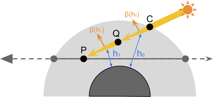
We calculate first the amount of light from that reaches  :
:
![\[I_Q = I_S \exp{\left\{-\beta{\left(\lambda, h_0\right)} \overline{CQ} \right\}}\]](https://www.alanzucconi.com/wp-content/ql-cache/quicklatex.com-bed106a65f8c0a1e2cb10230fa87ea31_l3.png "Rendered by QuickLaTeX.com")
Then, we use the same approach to calculate the amount of light that reaches from :
![\[I_P = \boxed{I_Q} \exp{\left\{-\beta{\left(\lambda, h_1\right)} \overline{QP} \right\}}\]](https://www.alanzucconi.com/wp-content/ql-cache/quicklatex.com-f407f4c9bae5534c63499f9e227f95c0_l3.png "Rendered by QuickLaTeX.com")
If we subsitute  in the second equation and simplify, we get:
![\[I_P = \boxed{I_S \exp{\left\{-\beta{\left(\lambda, h_0\right)} \overline{CQ} \right\}}} \exp{\left\{-\beta{\left(\lambda, h_1\right) \overline{QP} \right\}}=\]](https://www.alanzucconi.com/wp-content/ql-cache/quicklatex.com-dd69421f59879105164dfc73961f94e5_l3.png "Rendered by QuickLaTeX.com")
![\[=I_S \exp{\left\{-\beta{\left(\lambda, h_0\right)} \overline{CQ} -\beta{\left(\lambda, h_1\right) \overline{QP} \right\}}\]](https://www.alanzucconi.com/wp-content/ql-cache/quicklatex.com-0dd07ececa2b75ca7bf2242fa5cc4d7e_l3.png "Rendered by QuickLaTeX.com")
If both and have same length  , we can further simplify our expression:
![\[I_P=I_S \exp{\left\{-\boxed{\left({\beta{\left(\lambda, h_0\right)} +\beta{\left(\lambda, h_1\right)\left) ds} }} \right\}}\]](https://www.alanzucconi.com/wp-content/ql-cache/quicklatex.com-9ebcb8157b87bd2b536b76bf1b2abb9d_l3.png "Rendered by QuickLaTeX.com")
In the case of two segments of equal length with different scattering coefficients, the out-scattering can be calculated by summing up the scattering coefficient of the individual segments, multiplied by the segment lengths.
We can repeat this process with an arbitrary number of segments, getting closer and closer to the actual value. This leads to the following equation:
![\[I_P = I_S\exp\left\{ -\boxed{ \sum_{Q \in \overline{CP}} { \beta\left( \lambda, h_Q \right) } \, ds } \right \} \]](https://www.alanzucconi.com/wp-content/ql-cache/quicklatex.com-b905c9ea8533efb981594e6b6933ca08_l3.png "Rendered by QuickLaTeX.com")
where  is the altitude of the point .
The approach of splitting a line into multiple segments just like we have done is called numerical integration.
If we assume that the initial amount of light received is equal to , we obtain the equation for the atmospheric transmittance over an arbitrary segment:
![\[T\left(\overline{CP}\right) =\exp\left\{ -\sum_{Q \in \overline{CP}} { \beta\left( \lambda, h_Q \right) } \, ds \right \} \]](https://www.alanzucconi.com/wp-content/ql-cache/quicklatex.com-f72c2f0d566c33499588c0944b8234a6_l3.png "Rendered by QuickLaTeX.com")
We can further expand this expression by replacing the generic with the actual value used by the Rayleigh scattering, :
![\[T\left(\overline{CP}\right) =\exp\left\{ -\sum_{Q \in \overline{CP}} { \boxed{\frac{8\pi^3 \left(n^2-1 \right )^2}{3} \frac{\rho\left(h_Q\right)}{N} \frac{1}{\lambda^4}} } \, ds \right \} \]](https://www.alanzucconi.com/wp-content/ql-cache/quicklatex.com-8b74c7ad117f46cc1a67a39d281a6d74_l3.png "Rendered by QuickLaTeX.com")
Many factors of are constant and can be factored out of the summation:
![\[T\left(\overline{CP}\right) =\exp\left\{ - \underset{\beta\left(\lambda\right)}{ \underset{\text{constant}}{ \underbrace{ \frac{8\pi^3 \left(n^2-1 \right )^2}{3} \frac{1}{N} \frac{1}{\lambda^4} }}} \overset{\text{optical depth}\,D\left(\overline{CP}\right)}{ \overbrace{ \sum_{Q \in \overline{CP}} { \rho\left(h_Q\right) } \, ds}} \right \}\]](https://www.alanzucconi.com/wp-content/ql-cache/quicklatex.com-078c7de030885675fd00e0d337d08060_l3.png "Rendered by QuickLaTeX.com")
The quantity expressed by the summation is referred to as optical depth  , and is what we will actually calculate in the shader. The remaining part is a multiplicative coefficient which can be calculated only once, and corresponds to the scattering coefficient at sea level. In the final shader, we will calculate only the optical depth, and provide the scattering coefficients at sea level as an input.
To sum it up:
![\[T\left(\overline{CP}\right) =\exp\left\{ - \beta\left(\lambda\right) D\left(\overline{CP}\right) \right\}\]](https://www.alanzucconi.com/wp-content/ql-cache/quicklatex.com-0cb5b2489753c354c112f588e7b67f09_l3.png "Rendered by QuickLaTeX.com")
If you are interested in this topic, I would also suggest reading Carl Davidson post on atmospheric scattering, where he used an improved version of this iterative approach.
Coming Next…
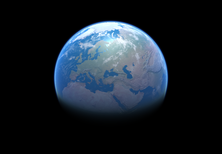
This post explained how to model Earth’s atmosphere. With the next post, we will start writing the shader code necessary to simulate atmospheric scattering.
You can find all the post in this series here:
- Part 1. Volumetric Atmospheric Scattering
- Part 2. The Theory Behind Atmospheric Scattering
- Part 3. The Mathematics of Rayleigh Scattering
- Part 4. A Journey Through the Atmosphere
- Part 5. A Shader for the Atmospheric Sphere
- Part 6. Intersecting The Atmosphere
- Part 7. Atmospheric Scattering Shader
- 🔒 Part 8. An Introduction to Mie Theory
Download
Become a Patron!
You can download all the assets necessary to reproduce the volumetric atmospheric scattering presented in this tutorial.
| Feature | Standard | Premium |
| Volumetric Shader | ✅ | ✅ |
| Clouds Support | ❌ | ✅ |
| Day & Night Cycle | ❌ | ✅ |
| Earth 8K | ✅ | ✅ |
| Mars 8K | ❌ | ✅ |
| Venus 8K | ❌ | ✅ |
| Neptune 2K | ❌ | ✅ |
| Postprocessing | ❌ | ✅ |
| Download | Standard | Premium |
💖 Support this blog
This website exists thanks to the contribution of patrons on Patreon. If you think these posts have either helped or inspired you, please consider supporting this blog.
📧 Stay updated
You will be notified when a new tutorial is released!
📝 Licensing
You are free to use, adapt and build upon this tutorial for your own projects (even commercially) as long as you credit me.
You are not allowed to redistribute the content of this tutorial on other platforms, especially the parts that are only available on Patreon.
If the knowledge you have gained had a significant impact on your project, a mention in the credit would be very appreciated. ❤️🧔🏻
Hi Alan!
I just supported you on Patreon, but I can’t seem to figure out how to access to the tutorial, where should I put the password? Could you please help me on this?
Thanks,
Toni
Hi Toni!
First of all, thank you!
I have recently switched to the Patreon API, but it seems they are not working.
Other people have been unable to access the tutorial. 🙁
I am switching back to the previous system.
If you are a $5+ patron, you should be able to access the entire series from here: https://www.patreon.com/posts/14814109 !
Let me know if you’re experiencing any other issue, and thank you for your patience!
Hi Alan!
Thank you for the quick support, now I can access to the tutorials! 🙂
Toni
In the tip Where does exp come from, I dont understand why in the limit expression ,the bottom number is n not 2? The process is I0*(1-β/2)*(1-β/2)*(1-β/2)*(1-β/2)….so the result is I0*(1-β/2)^n,isnt it? I am unfamiliar with Calculus,so can you say more about this ? Or you can give me some link about Calculus that help me to understand this. Thank you very much!
I think I understand what you mean!
To get CLOSER to the real value, we first do an approximation using TWO steps.
So we take the value, we multiply it (1-β/2) and then what remains by (1-β/2).
Here the /2 is added because we repeat the process twice, so we half the contribution of each multiplication by two to compensate.
Then, we can do the same to get an even more precise value, by repeating the process THREE time. But this time we divide β by 3. So it is (1-β/3)*(1-β/3)*(1-β/3).
Here we repeat the process three time, so we divide each by 3 to compensate.
Then we repeat 4 times, 5 time, …etc.
If we use the limit, we can effectively apply (1-β/n) exactly n times, with n that goes to infinity.
thanks,but i want to know more detail about “exp come from”,what should i do?
If you click on it, it will expand a section explaining how exp is derived!
I dont understand the “exp{x}”,what does this meaning?