Voronoi Diagrams

This tutorial is a primer on Voronoi diagrams: what they are, what you need them for and how to generate them using a Shader in Unity. You can download the complete Unity page in Part 4.

Part 1: Voronoi Diagrams

Technically speaking, Voronoi diagrams are a way to tassellate a space. It means that the end result of Voronoi is a set of “puzzle pieces” which completely fills the space. To start, we need a set of points (often called seeds) in the space. Each seed will generate a piece of this puzzle. The way Voronoi works is by assigning every point of the space to its closest seed. The final result heavily depends on the way distance is measured in the space.

Euclidean distance

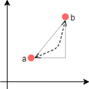
Most Voronoi diagrams are are based on the Euclidean distance. The cost between two points is given by the length of the shortest segment which connects them both. It can be calculated easily with the Pythagorean theorem:

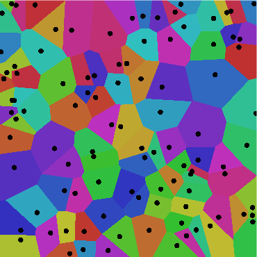
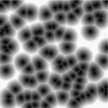
In Cg, this function is already implemented and is called distance. The picture on the left shows a Voronoi diagram based on the Euclidean distance, drawn with 100 points. On the right, the same diagram uses a gradient to visualise the actual distance from a pixel to the closest one.

Manhattan distance

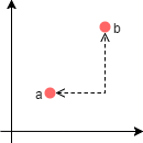As the name suggests, the Manhattan distance takes his name from the homonym city. The shortest path between two locations is not a straight line, since Manhattan is full of buildings. The shortest distance is the one which goes around building.

half distance_manhattan(float2 a, float2 b) {
	return abs(a.x - b.x) + abs(a.y - b.y);
}

Compared to the Euclidean distance, It is sensibly less expensive to calculate.

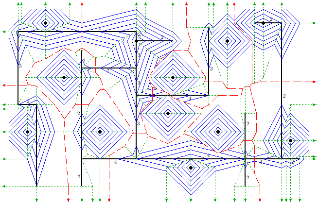
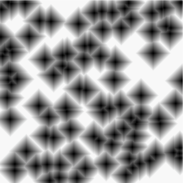
Using the Manhattan distance produces very intriguing patterns which resemble circuit boards. This is not a coincidence: many boards are designed to minimise circuit length and avoid curves.

Minkowski distance

Despite looking very different, both the Euclidean and the Manhattan distances are both special cases of a more general metric: the Minkowsi distance. To understand why, you have to remind some algebra. In the same way multiplication and division are the same operator (dividing by is equivalent to multiply by ), even root and exponentiation are deeply connected. Remembering then , we can introduce the Minkowski distance:

When or  it equivalent to the Manhattan or Euclidian distance, respectively.

half distance_minkowski(float2 a, float2 b, float p) {
	return pow(pow(abs(a.x - b.x),p) + pow(abs(a.y - b.y),_P),1/p);
}

The most fascinating aspect is that is provides a way to smoothly transitioning from the Euclidean to the Manhattan distance, and the other way round.

 If you are in a higher dimension, the Minkowski distance can be still used, providing that you calculate it on all the components of two points and :

Applications

Part 2: Applications

Despite looking pretty, not a single application has been indicated for Voronoi diagrams yet. In actuality, they play a very important role in Science, and many games can benefits from them.

In games

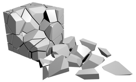
Breaking object realistically is a very challenging task, that requires to know how pressure waves propagates through a material. A simpler way to create plausible fractures in an object is to rely on a Voronoi 3D tassellation. You start choosing random points within the object you want to break, then each Voronoi cell become one of its chunks. In games, breakable objects don’t break: they are already broken, and your interaction makes the piece falling apart.

The famous Fracturing & Destruction plugin on the Asset Store, for instance, uses this technique to generate breakable objects. A future post will show how to replicate this effect at no cost.

In path finding

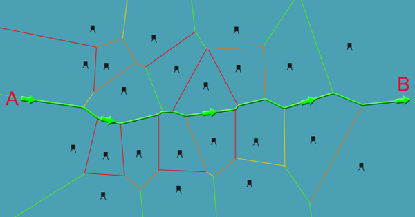
As a game developer, you might be familiar with path finding. A* is notoriously the most known, but there are many other ways one can find the optimal path between two points. So far, Voronoi diagrams have been seen as independent regions of space although there is an alternative way of interpreting them. If we put a node every time two segments connects, Voronoi produces a graph. The segments (now edges of the graph) represent the paths which are as far as possible from the seeds. In terms of gaming, seeds can be enemies you want to avoid; travelling on the edges provides the safest route possible. Brent Owens has written a very nice tutorial about this.

Conversely, Voronoi diagrams can be also used to approximate the shortest path. The dual graph of a Voronoi diagram (known as the Delaunay triangulation) allows to find paths which are as close as possible to the seeds. When coupled with the Manhattan distance, it can be used to generate the fastest route within a city, considering how fast you can go on different roads.

In nature

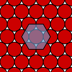Circle packing is the problem of fitting as many circles as possible in a given space. The best possible solution to this problem is shown on the left; circles are arranged in a hexagonal lattice, which resemble a honeycomb. This is actually why honeycomb cells have a hexagonal structure: if all circle expands at the same time to fill all the space around them, they’ll end up pressing against each other until they create a perfect hexagonal lattice. The same pattern can be found in several other phenomena, like cooling magma and soap bubbles. The latter, provide an excellent (and transparent) example of how Voronoi diagrams look in three dimensions.

The next part of this tutorial will show how to generate Voronoi diagrams using Shaders.

Generation

Part 3: Generation

There are several algorithms you can rely on to generate Voronoi diagrams.  Every point is independent from the other, so this is one of those perfect applications for a shader. Traditionally the Fortune’s algorithm (left) is commonly used, but it is very hard to implement within a shader. The tricky part, in this case, is how to provide a list of points to the Material, since the Unity APIs don’t provide any SetArray function. Luckily, there is an undocumented feature you can use to pass arrays and matrices to a shaders, and it has been discussed in this post. We will use one array for the position of the points (in a 2D space) and another one for the colours. A variable called _Length is used to indicate how many points are there since Cg doesn’t support arrays of arbitrary dimensions.

uniform int _Length = 0;
uniform half2 _Points[100];
uniform fixed3 _Colors[100];

The actual code of the Voronoi diagram is implemented in the fragment function. For each pixel, it simply loops over all the points and finds the closest one. Its index is then used to find the right colour to use:

fixed4 frag(vertOutput output) : COLOR {
	half minDist = 10000; // (Infinity)
	int minI = 0;
	for (int i = 0; i < _Length; i++) {
		half dist = distance(output.worldPos.xy, _Points[i].xy);
		if (dist < minDist) {
			minDist = dist;
			minI = i;
		}
	}
	return fixed4(_Colors[minI], 1);
}

half4 color = tex2D(_RampTex, fixed2(minDist, 0.5));
color.a = 1;
return color;

Weighted Voronoi diagrams

Interesting results can be obtained by mixing different metric, or altering the “attraction” of the seeds by providing an extra coefficient to the shader. The distance is now:

half dist = distance(output.worldPos.xy, _Points[i].xy) + _Weights[i];

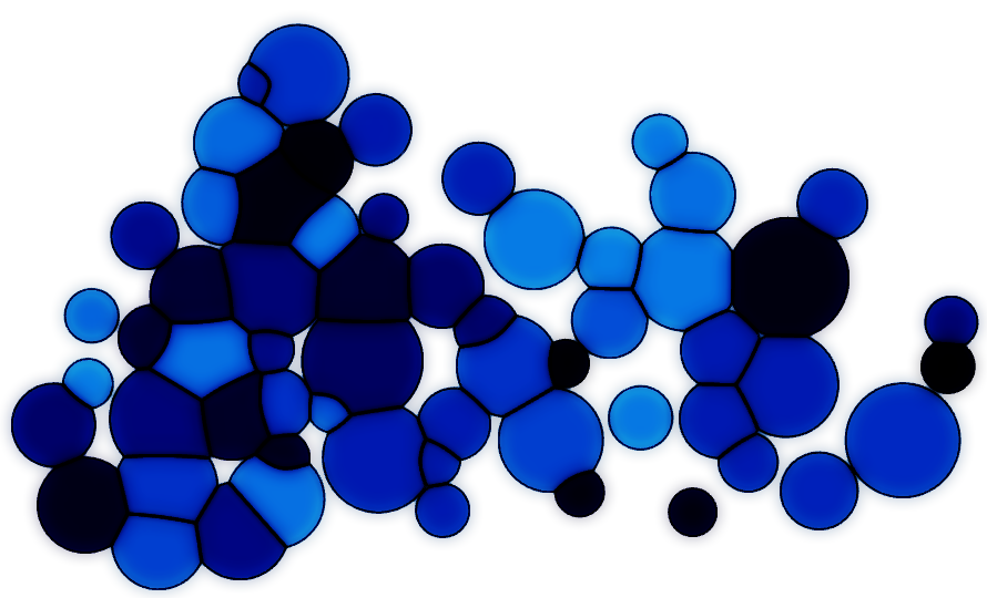
This takes the name of weighted Voronoi (also known as Dirichlet tessellation) and it can be used to generate beautiful effects, like Milan Domkář did with his foam:

Cone projection

There is a smarter approach to generate Voronoi diagrams (almost!) for free, and Chris Wellons is beautifully explaining it in its blog. You can generate a Voronoi tessellation by projecting cones out of the starting points. The cones will eventually intersect and seeing them it from the above will produce the same effect.

You can download the full Unity package in the last part of this tutorial.

Conclusion & Download

Conclusion

Voronoi diagrams are a way to tessellate the space which has many applications, from game development to city planning. This tutorial has shown how to generate them using a shader; you can download the complete Unity package here.

Other resources

• How to Use Voronoi Diagrams to Control AI: How Voronoi diagrams can be used to create very good AIs which avoids enemy;
• Pathing Excursions: A way to create very realistic AIs which can patrol around buildings;
• A GPU Approach to Voronoi Diagrams: How to render Voronoi diagrams on the GPU, in a very smart way;
• Voronoi Diagram for the City-Metric: Voronoi diagrams applied to city planning;
• foam: a bubble-like lattice created using weighted Voronoi diagrams.
• Voronoi Diagrams on the GPU