
This is the second part of the series dedicated to one of the most popular sensor de-noising technique: Kalman filters. This article will introduce the Mathematics of the Kalman Filter, with a special attention to a quantity that makes it all possible: the Kalman gain.
You can read all the articles in this online course here:
- Part 1. A Gentle Introduction to the Kalman Filter
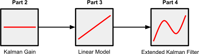
- Part 2. The Mathematics of the Kalman Filter: The Kalman Gain
- Part 3. Modelling Kalman Filters: Liner Models
- Part 4: The Extended Kalman Filter: Non-linear Models
- Part 5. Implementing the Kalman Filter 🚧
Introduction
Kalman filtering is a very powerful technique that finds application in a vast number of cases. One of its most popular use is sensor de-noising. Readings from sensors are typically affected by a certain degree of statistical uncertainty, which can lead to poor measurements. Under certain circumstances, Kalman filters have been proved to be optimal, meaning that no other algorithm will perform better.
This series of tutorials aims not just to explain the theory behind Kalman filters, but to create a fully functioning one! Many books present the equations in their “final” form; while that is a very time-efficient approach, it is not the one that we have chosen for this series.
If we want to understand not just how Kalman filters work, but why they work, it is important to do so step by step. And so, this series will build a Kalman filter “iteratively”, adding a new features at the end of every article.
By the end of this first article—which will focus on a quantity called Kalman gain—we will have a fully-functioning Kalman filter which is able to de-noise signals that are not expected to change very rapidly.
The following part will extend this limitation, but introducing a much more “complete” version of the Kalman filter which can handle signals that evolve linearly over time.
Finally, another article will introduce the so-called Extended Kalman Filters, which are designed to handle signals that can evolve in more complex ways.
How it Works
When it comes to Kalman filters, most online tutorials start with the example of a moving train. The position of the train at a given time  —let’s call it
  —is the unknown property that we want to estimate. If we had direct access to the true position of the train, there would be no need for Kalman filters. The only way to access the position of the train is indirectly, by some sort of measurement; for instance, a GPS. If we had a truly perfect GPS, there would be no need for Kalman Filters. Unfortunately, no measurement apparatus is perfect, and no matter what we do, our measurement—let’s call it
  —will always be affected by noise, errors and inaccuracies.
From a mathematical point of view, we can model this in the following diagram:

The train (generally referred to as the process) changes its position at every new time interval. This is often referred to as process update. In an ideal scenario, if a train travels at a constant speed of  metres per second, it yields the following relationship:
(1) 
where  is the difference in time between two updates.
Each measurement () will be close to the actual position (), plus or minus some random noise (more on that later). When the system starts,  is the first (and only) measurement taken. Consequently, it is also our best guess on the real position of the train,
  . The “best guess” for the real position of the train, often referred to as the estimated position, is indicated at
  . When the system starts, the first measurement is also the best estimated position at time
  :
:
(2) 
What a Kalman filter does, is updating and refining the estimated position () as the system evolves. And it does so by integrating (fusing) together the information about where the system believes the train should be () and where the measurement tells it is ().
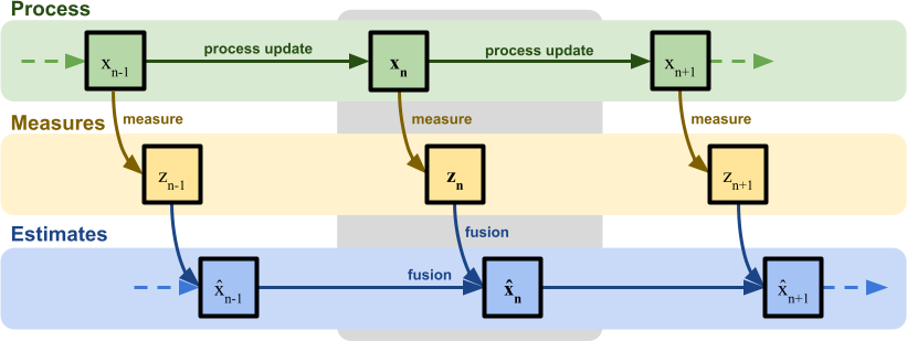
Both quantities are inherently inaccurate, but combining them both can help refining the overall estimate. In this example we used two measures, but this can theoretically be expanded to include more readings from different sensors, all of which having different degrees of reliability. This is commonly known in the academic literature as sensor fusion.
The rest of this article will slowly expand on this simplistic interpretation of Kalman filtering, by progressively introducing more nuanced variants.
Step 1: The Model
Each Kalman filter is tailored to the application it needs to be used for, and it does so by incorporating a model of the system. This model is a simplified mathematical description of how we expect the system to evolve. In the case of a train, the Kalman filter would need to integrate the laws of motion into its equations. This allows the filter to not just passively reacts to the train movement, but to predict its future position based on its current state. Equation (1), for instance, is modelling the fact that the train position increases linearly with time.
It is important to understand two things about this:
- This is a belief: all Kalman filters are built with some pre-existing knowledge of how the system should evolve. The idea that the train moves at a constant speed is a belief, which may or may not be entirely correct;
- This is a model: the Kalman filter does not expect (or require) (1) to be valid at all times. That equation is a simplified model of how the system is expect to behave at a short time scale. As such, there is no requirement for this to be exact. The more precise the model can be, the better the system will react. But because Kalman filters are designed to be resilient to noise, errors or inaccuracies in the model are generally well tolerated, as their deviation from the “true” behaviour can simply be interpreted as an extra source of noise.
This leads to an algorithm that works in two separate steps:
- Time update (or prediction step): based on the current state of the system, we predict its new state.
In the case of a train, this means predicting its next position based on its previous position and previous velocity. - Measurement update (or correction step): the prediction generated in the step before is corrected using the data from a sensor.
In the case of a train, this means integrating the predicted position with the measurement from a GPS.

Under this framework, the expected position updated in the prediction step is called a priori state estimate ( ). “a priori” means “before“, as this is the predicted position where the train should before the measurement is performed. Once a measure is available, the Kalman filter can integrate that information to refine its estimation, which gets called a posteriori state estimate.
📡 What if sensors readings are not always available?
The need for a model which explains how the process we are analysing is evolving (i.e.: how the train moves over time) becomes very important when we consider one real constraints that all sensors have: delay.
In a realistic setting, in fact, it is very unlikely to have instantaneous access to a sensor measurement at every time frame. GPSes, for instance, take a very long time to be queried; time during which the system is still evolving (to be read: the train is still moving even when you are not measuring it!).
Having an internal model of how the system should update from one time frame to the next one, allows to simulate its evolution even when there are no measures readily available.

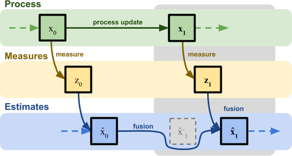
In the example above, for instance,  is equal to
  , since no correction step takes place.
A simpler toy example
Most online tutorials start with the example of a train moving forward along a track; and this tutorial was not an exception. Such a scenario is very easy to understand. However, when it comes to the actual Maths, following such a path actually leads to a more complex derivation. This is because each Kalman filter is tailored to the application it needs to be used for, and doing so requires to integrate the laws of motion into our equation. And doing so, “pollutes” the derivation of the Kalman filter by adding specific terms that are not part of the filter itself, but of the model the filter is trying to predict.
In this specific article, we will focus only on the correction step, which is the real heart of the Kalman filter; something that all filters belonging to Kalman family share. But for this to work, we need to pick a scenario in which the prediction step is virtually non-existent. This means measuring a quantity that is not expected to change over time. More realistically, a quantity that is not expected to change too fast. This leads us to consider a system which was already described in the second diagram of this article:
A good example is the temperature of a well-insulated room. Let’s assume that the real temperature at time is equal to . Under our assumption, we believe that the system evolves according to the following equation:
(3) 
This means that we expect the temperature of the room to remain constant, as the room itself is well insulated.
Also, to simplify the notation—yet without loss of generality—we will only consider the evolution of the Kalman filter from a generic time  to
to  :
:
This has no real implication, but it allows to simplify the notation getting rid of  , and
, and  subscripts.
🌡️ The concept of temperature is a statistical one!
For the ones of you who want to be very pedantic, the concept of temperature is not a “inherent” property of a system: it is a statistical one. Temperature is ultimately determined by the average kinetic energy between atoms, constantly bouncing off each other. Under this definition, temperature itself is not a constant property, but one that keeps changing as the energy in the system gets exchanged with the sensor.
However, for this toy example, we will not bee too worried about this, and imagine temperature to be a constant value.
Step 2: The Measurement
If we could access the real temperature of the room () at any arbitrary time (), we would have no need for a Kalman filter. The problem is that we can never sample the temperature directly and with absolute precision. Instead, we are forced to rely on an indirect, imprecise measure, which introduces some uncertainty. What we read from a thermometer is not a value of the “real temperature”. It is (to make an old-fashioned example) how much mercury expands when subjected to a certain temperature. The expansion of mercury is a proxy for the temperature, which is the real quantity that we want to estimate.
Measuring the temperature of a room using a thermometer introduces a new type of uncertainty, as the sensor itself has a limited precision.
(4) 
(5) 
The quantity  represents the temperature reading at the time
  , which is a function of the actual temperature
  plus some uncertainty modelled by the Gaussian variable
  , referred to as the measurement noise.

The quantity  measures how reliable the sensor is. You can calculate experimentally, simply by querying the sensor many times and measuring the variance of its output. In our example, however, we assume it is constant throughout the entire life of the filter. This is not always the case; the precision of a GPS, for instance, depends on how fast you travel. Likewise, it is fair to assume that the precision of a thermometer could be a function of the temperature.
Visualising Noise and Uncertainty
Before we proceed, you should be familiar with the concept of Gaussian distribution. To get a better idea of the true meaning of (4) you can have a look at the interactive chart below. The blue curve shows the probability density function of ; for its value on the X axis, it indicates its relative likelihood of appearing.
|
–
|
|
|
–
|
If the sensor returns the value , it does not mean that the temperature really is . Its probability density function shows how likely the other temperatures are.
🔔 Tell me more about the Gaussian distribution!
When you are rolling a dice, there are six possible outcomes: one for each face. Statistically speaking, we say that rolling a die is a random process. Assign the variable  to this process means that can assume any value from the set
  . For a standard dice, each value is equally likely. This means rolling a dice is a random process with uniform distribution.
Certain processes follow a different distribution, meaning that the different values generally have different probabilities of being selected. One very special distribution is the Gaussian distribution, also called the normal (because it naturally occurs in many phenomena) or bell curve (due to its bell-like shape).
Intuitively, saying that  follows a Gaussian distribution means that it is a random variable, and that large deviations from its mean value are less likely than small ones. The rest of the derivation requires a solid understanding of Gaussian distributions; if you are unfamiliar with the concept, Understanding the Gaussian Distribution is a good starting point.
❓ How come the curve can go above 1?
The curve seen in the interactive chart above represents the probability density function of the Gaussian variable . Probabilities must always be confined to the interval ![\left[0, 1\right]](https://www.alanzucconi.com/wp-content/ql-cache/quicklatex.com-ac0ef5000a04390b73f0f437f914143d_l3.png "Rendered by QuickLaTeX.com") , so it might sound weird to see the pdf assuming values greater than .
, so it might sound weird to see the pdf assuming values greater than .
Conversely to what it might seem, the value of the pdf at an arbitrary point does not represent the probability of that point. The value of the pdf above at  is approximately
  ; this does not mean that has a 39% chance of being . We can see why this line of reasoning fails by imagining a dice: each face has probability
  of being chosen because there are
  sides. The random variable is a continuous variable; the probability of any single value is technically , because there are infinitely many to choose from.
The value generated by a pdf cannot be used to estimate absolute probabilities. It can, however, be used to estimate relative probabilities. The point  has pdf approximately equal to
  . Since this is half the value that had at , it means that is twice as likely to be selected compared to
  .
.
Step 3. Estimated Position
The purpose of sensor de-noising is, at its core, finding a good guess for , based on the information we have previously collected, and on any available sensor reading. This guess is often indicated in the scientific literature as  and is called the estimated state (or position, in our example) at time . When it comes to reading sensors, the most simple approach is to blindly trust them. Which means saying that
  . Very often, this is also the worst approach you can take. Every sensor reading comes with a certain degree of uncertainty, and relying on its raw value means that you are comfortable integrating the maximum amount of noise possible into your application.
A more reasonable approach is to come up with a different equation for . One that, for instance, takes into consideration not just the most recent reading from the sensor, , but also how hot we believed the room was one instant ago. This takes the form of the estimated position at the previous time , which is called  . By relying on both pieces of information we are implying that the actual position should not be too far from where the train was before.
There are infinitely many ways in which and can be merged together. The simplest way is simply to combine them linearly:
(6) 
Equation (6) interpolates between and linearly, using the coefficient ![k_1\in\left[0,1\right]](https://www.alanzucconi.com/wp-content/ql-cache/quicklatex.com-43f560705299e3cdde1c912f25f1aa68_l3.png "Rendered by QuickLaTeX.com") . When
. When  , we return to the case in which we fully trust the sensor and we have that . When
  , instead, we weight the sensor and our previous guess equally and the new position is simply the average of the two:
  . If we assume
  , we are implying that the sensor is not to be trusted, and its contribution is simply ignored.
What we have done here is called linear interpolation: a technique that all game developers should be very familiar with. In case you are interested to learn more about what it can do and how it can be used, An Introduction to Linear Interpolation is a good starting point.
It is obvious at this point that, if we decide to mix and linearly, the coefficient  indicates how much trust we have in the raw value obtained from the sensor. The interactive chart below shows a Kalman filter designed for signals that are not expected to change over time. You can try changing the value of the Kalman gain (
 ) to see how the filter adjusts itself.
|
0.08
|
|
|
0.1
|
You can obviously choose the value of by hand, but what Kalman does is finding, at each time step, its optimal value. The term “optimal” means that, under the right conditions and providing certain assumptions are holding, it converges to the the value of so that the estimated position is as close as possible to the actual position .
❓ Deriving Kalman Filter using Least Squares Minimisation
There are countless derivations of the Kalman filter. If you studied Maths at a College level, you might already have an idea of how to solve this problem. Finding the best value for is, at its heart, an optimisation problem. In fact, one can imagine the following quantity:
(7) 
which measures the error in the filter estimation of the room temperature, against the real one. If we replace with (3), with (6) and with (4), we obtain the following expression:
(8) 
which reveals that even the error  can be expressed as a liner combination between the previous error (
 ) and the measurement noise ():
(9) 
Finding the optimal value for means finding the value in the interval ![\left[0,1\right]](https://www.alanzucconi.com/wp-content/ql-cache/quicklatex.com-e2b4c064b644035fc625f8ca9afa5f3a_l3.png "Rendered by QuickLaTeX.com") for which is minimised. If was a traditional function, you could calculate its derivative according to to find its root. However, is a random variable and such an approach will not work since the expression does not have a fixed value, but it changes every time.
for which is minimised. If was a traditional function, you could calculate its derivative according to to find its root. However, is a random variable and such an approach will not work since the expression does not have a fixed value, but it changes every time.
A typical approach to minimise random variables is a method called least squares, which minimises the mean (also called expected value and represented by ![E\left[\cdot\right]](https://www.alanzucconi.com/wp-content/ql-cache/quicklatex.com-41f4366f3333cd6c30533a98fcc9dde9_l3.png "Rendered by QuickLaTeX.com") ) of the squared error:
) of the squared error:
(10) ![\begin{equation*} E\left[e_1^2\right] \rightarrow min\end{equation*}](https://www.alanzucconi.com/wp-content/ql-cache/quicklatex.com-60c9386dbf48f327ab7d005dbbf2fbdf_l3.png "Rendered by QuickLaTeX.com")
This allows finding an optimal value for , and is often one of the most common ways in which the equations for the Kalman filters are derived. For a complete derivation, you can read David Khudaverdyan‘s article titled “Kalman Filter“.
Step 4. Sensor Fusion
To understand how Kalman finds the optimal value for , we have to take a step back to talk about probability distributions. Every random process has a probability density function (or pdf), which indicates the values it can produce, and how likely they area.
In the case of the thermometer that is used in this example, we have assumed the pdf of its error to follows a Gaussian distribution. When the sensor reads a value of , we know there is an uncertainty associated with that value which can be modelled as generated from a Gaussian distribution with variance , as seen in (4). Incidentally, this means that if we assume the sensor noise to be normally distributed, we can also model the sensor reading itself () as sampled from a normally distributed variable. Let’s call it  :
:
(11) 
which means that the value returned by the sensor () is not perfect.
What we are trying to do here is to model all parts of the system as normal distributions. This will allow us to borrow the much needed statistical tools which will help compensating for the presence of noise.
This was pretty much straightforward for (), since its normal distribution was a direct consequence of assuming the sensor noise followed a normal distribution in the first place. But we cannot simply assume the same for the various . This is because the estimated states are the result of an iterative process, which combines the current sensor reading with the previous state estimate. But as we can clearly see from (6), is a linear combination of two normally distributed variables. As we have just discussed, is normally distributed; and as it turns out, is normally distributed as well! This is definitely true in its very first iteration, where  , as seen in (2). In the following iteration, will be a linear combination of (normally distributed) and (normally distributed, as ). A linear combination of two normally distributed variables has a normal distribution. Following this very reasoning, every instance of is normally distributed, as it is a linear combination of two normally distributed variables.
Thanks to this inductive reasoning, even the estimated temperature () can be modelled as if it was sampled from a Gaussian distribution (let’s call it  ), as its value comes with a certain degree of uncertainty. While the variances of the process and measurement noises,
  and are inputs of the Kalman filter (i.e.: they are not assume to change over time), the variance of is a quantity that depends on time and that that we will need to calculate. For now, let’s call it
  , so that the probability distribution of can be expressed in the form:
(12) 
Practically speaking, indicates the overall confidence over the estimated position , sampled from the random variable . While the variance of the measurement noise stays the same throughout the entire life of the filter, the confidence on our estimated position changes over time. It makes sense to update not only our estimated position to , but also how confident we are about its accuracy from to  . We expect the Kalman filter to converge to the real temperature of the room pretty quickly, so it means that its confidence should increase over time. On the other hand, if the temperature is subjected to a sudden change, it might take some time for the filter to recover and we should trust its current estimate less.
Joint Probability
We now have two different probability distributions, each one estimating the probability of finding how hot the room is. These distributions are not only associated with a mean (which is their best guess), but also with a variance that indicates how confident that guess is. Their joint probability is a new probability distribution which incorporates all of these pieces of information.
What Kalman does is finding the most likely estimation for the temperature of the room, calculating the joint probability of the two distributions, and , effectively finding the distribution for the new estimate of the room temperature,  .
.
If we assume and to be independent of each other, their joint distribution can be found multiplying them together:
(13) 
One of the things that make the derivation of the Kalman filter algorithm so clean and efficient is that the product of two Gaussian distributions is another Gaussian distribution:
(14) 
This means that the process can be repeated indefinitely, without increasing in complexity. And it is, ultimately, what allowed us to assume that even the estimated position () was following a normal distribution, as seen in (12).
❓ Show me the derivation!
The solution can be found by multiplying together the probability density functions of the two Gaussian distributions.
You can read the complete derivation in the article “Products and Convolutions of Gaussian Probability Density Functions” by P. A. Bromiley.
We can use (14) to multiply together the probability distributions of and :
(15) 
Before progressing, is important to understand what this means, in the context of our example. Both and are different measures of the temperature of the room. They are affected by a random error, so we assume they are sampled from two Gaussian distributions: and , respectively. Their joint distribution, takes into consideration not only the distribution means ( and ), but also how confident these values are (represented by their variances, and ). Since the mean of a Gaussian distribution is the value that is most likely to occur, the mean of the joint distribution () will be the most likely temperature of the room at time . Reframing the problem in terms of probability density functions, (15) also allows to derive the variance of , called , which indicates how confident we are in its accuracy.
Step 5. The Kalman Gain
If we look at the new definition that we have derived for from (15), it looks quite different from what originally proposed in (6). In reality, they are indeed the same quantity, although just expressed in a different way. We can see this by rearranging (15) like this:
(16) 

There is a hidden beauty in this derivation, which arises from the fact that a probabilistic definition of the problem, based on two Gaussian distributions and , simplifies into a linear interpolation between and . When expressed in this form, the coefficient is called the Kalman gain:
(17) 
Now we have all the pieces to calculate the temperature of the room , based on the previous estimate and the current data from the sensor . This derivation also provides an additional quantity which can be used to measure the confidence in our result.
To recap:
(18) 
❓ How come Least Squares and the joint probability converge?
This article has shown two approaches to derive the Kalman filter. One using Least Squares on the estimation error , and one using the joint probability of the two random variables associated with the previous estimated temperature and the sensor measurement .
These two approaches are completely different, yet they converge to the same result. This is not a coincidence. According to the Gauss-Markov Theorem, there is a deep connection between Least Squares and Gaussian noise. Loosely speaking, minimising a random variable using least squares is implicitly assuming that it has a Gaussian distribution.
In the context of Least Squares, the term Gaussian noise is often replaced by spherical noise.
Step 6. Iterate
This derivation for the Kalman filter has been shown between an initial time and the following interval . In a real application, this process is repeated in a cycle.
Like any Mathematical model, the Kalman filter works under very strict assumptions. In this case, the evolution of the system has to be linear, the and measurement noise have to be Gaussian distributed. For this specific derivation, we have also assumed that the quantity we want to measure never changes.
Visualising The Kalman Filter
Understanding what the Kalman filter really does can be quite challenging at first. The interactive chart below allows controlling the parameters of the random variables which represent the sensor measurement and previous estimate . The result is the updated estimate , which turns out to be another Gaussian distribution.
|
–
|
|
|
–
|
|
|
–
|
|
|
–
|
Summary
This post introduced the mathematics of Kalman filter. This is a list of all the symbols and notations used:
- : the real temperature of the room at time ;
- : the measured temperature, which is the data collected from the sensor at time
 ;
;
This is a noisy estimate for the values of; - : the measurement noise, which indicates how reliable the sensor is.
This is the variance of the sensor;
- : the estimated temperature of the room at time .
This is an inaccurate guess for, and it is calculated by taking into account  and ;
and ;  : the Kalman gain, which represents the best coefficient to merge the estimated temperature and the sensor measurement;
 : the confidence of the estimated position.
This is the variance of the estimated temperature.
To simplify the notations, we have focused on two generic time intervals referred to as and .
The next part of this series will extend the equations here presented, so that the filter can work even if the temperature changes.


What’s Next…
You can read all the tutorials in this online course here:
- Part 1. A Gentle Introduction to the Kalman Filter
- Part 2. The Mathematics of the Kalman Filter: The Kalman Gain
- Part 3. Modelling Kalman Filters: Liner Models
- Part 4: The Extended Kalman Filter: Non-Linear Models
- Part 5. Implementing the Kalman Filter 🚧
Further Readings
- “Kalman Filter For Dummies” by Bilgin Esme
- “Kalman” by Greg Czerniak
- “Understanding the Basis of the Kalman Filter Via a Simple and Intuitive Derivation” by Ramsey Faragher
- “Kalman filter” by David Khudaverdyan
- “Kalman Filter Interview” by Harveen Singh
- “Kalman Filter Simulation” by Richard Teammco
- “A New Approach to Linear Filtering and Prediction Problems” by Rudolf E. Kálmán
Leave a Reply