Modelling Kalman Filters

This is the third part of the series dedicated to one of the most popular sensor de-noising technique: Kalman filters. This article will explain how to model processes to improve the filter performance.

You can read all the tutorials in this online course here:

Part 1. A Gentle Introduction to the Kalman Filter
Part 2. The Mathematics of the Kalman Filter: The Kalman Gain
Part 3. Modelling Kalman Filters: Liner Models
Part 4: The Extended Kalman Filter: Non-Linear Models
Part 5. Implementing the Kalman Filter 🚧

Introduction

Before we can extend the Kalman filter towards its full potential, it is important to do a quick recap of what was explored in the previous two articles of this series.

Kalman filters are a family of statistical techniques which find ample application in engineering to solve the problem of sensor de-noising and sensor fusion. All sensors, in fact, are affected by errors, delays and inaccuracies which can have a significant impact on the system in which they are integrated.

Typical examples of system in which Kalman filters find ample applications are refining the location of an object (such as a train using GPS data) or controlling a thermostat (using readings from a thermometer). In the field of games, they are really useful when it comes to read input data from controllers, accelerometers, gyroscope and webcams.

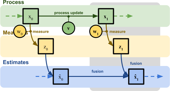
The theory of a Kalman filters sees the world through three different lenses:

The process: represents the system that we are trying to measure. The exact value of the system at time $n$ is $x_n$ . This value is never directly accessible, hence it must be sampled using a sensor;
The measures: they represents the raw data coming from a sensor. The reading of the system at time $n$ in $z_n$ . This reading is assumed to be affected by an additive noise factor, $w_n$ , which follows a normal distribution with variance $R$ ;
The estimates: they represents the guesses of the Kalman filter. The “best guess” for the value of the system ( $x_n$ ) at time $n$ is $\hat{x}_n$ . As a consequence of assuming that the various measurements are following a normal distribution, even the various $\hat{x}_n$ are normally distributed.

The diagram below summarises all of those elements. For simplicity, we will mostly refer to two generic time instances $n=0$ and $n=1$ :

The Kalman filters estimates the “true” value of the system by combining (fusing) together the best estimate of its previous value ( $\hat{x}_0$ ) with the latest measurement from the sensor ( $z_1$ ), in what is known as the state estimate (sometimes also referred to as the estimated position, when the filter is used for locations).

In one of its more vanilla implementations, this fusion is done by linearly interpolating $\hat{x}_0$ and $z_1$ based on the coefficient $k_1$ which is known as the Kalman gain.

(1) $\begin{equation*}\hat{x}_1 = \hat{x}_0 \left(1-k_1\right) + z_1 \, k_1\end{equation*}$

What the Kalman filter does is converging towards the optimal gain value: the value which results in the combination of the previous state estimate ( $\hat{x}_0$ ) and the current sensor measurement ( $z_1$ ) that best approximates the true value of the system ( $x_1$ ).

And it does so through a statistical approach. Because both quantities can be represented as being sampled from two normal distributions ( $\hat{X}_0 \sim \mathcal{N}(\hat{x}_0, P_0)$ for the previous state estimate $\hat{x}_0$ , and $Z_1 \sim \mathcal{N}(z_1, R)$ for the sensor reading $z_1$ ), the expected value of their joint probability distribution represents the best guess for the value of the system:

(2) $\begin{equation*} \mathcal{N}(\hat{x}_1, P_1)=\mathcal{N}(\hat{x}_0, P_0) \times \mathcal{N}(z_1, R)\end{equation*}$

In the previous article we made the example of a Kalman filter applied to a thermometer. In that scenario, we encountered the following quantities:

$x_1$ : the real temperature of the room at time $1$ ;

$z_1$ : the measured temperature, which is the data collected from the sensor at time $1$ ;
This is a noisy estimate for the values of $x_1$ ;
$R$ : the measurement noise, which indicates how reliable the sensor is;

(3) $\begin{equation*} z_1 = x_1 + w_1\end{equation*}$

(4) $\begin{equation*}w_1 \sim \mathcal{N}(0,R)\end{equation*}$

$\hat{x}_1$ : the estimated temperature of the room at time $1$ .
This is an inaccurate guess for $x_1$ , and it is calculated by taking into account $\hat{x}_{0}$ and $z_1$ ;
$k_1$ : the Kalman gain, which represents the best coefficient to merge the estimated temperature and the sensor measurement;

(5) $\begin{equation*} \hat{x}_1 = \hat{x}_0 \left(1-k_1\right) + z_1 \, k_1\end{equation*}$

(6) $\begin{equation*} k_1 = \frac{P_0}{P_0+R} \end{equation*}$

$P_1$ : the confidence of the estimated position $\hat{x}_1$ .

(7) $\begin{equation*} P_1 &= \left(1-k_1\right) P_0\end{equation*}$

Limitations

At this stage is important to remember that this series of tutorial is building a “fully functional” Kalman filter incrementally. The version presented in the diagram above works, but is still fairly simple compared to the more general versions that one would typically find in the scientific literature.

And yet, this is already enough to implement a fully working Kalman filter. The char below shows how the filter ( $\hat{x}_n$ , in blue) reacts to a static signal ( $x_n$ , in green) which is subjected to a sudden change:

$R$

0.08

The yellow line indicates the noisy measurements ( $z_n$ ), while the blue area represents the confidence of the filter its its own prediction ( $P_n$ ). This is plotted using its standard deviation ( $\sqrt{P}$ ), which here is greatly magnified to be better visible.

It is easy to see, however, that the filter’s performance is not that great. This is the results of an over-simplistic approach in its current derivation. In fact, there are two important aspects that so far have been ignored:

The process is believed to be static. The current iteration of the Kalman filter presented assumes that the true state of the system is typically not subjected to any change over time. For instance, the location of a building is not supposed to change over time. While this is true in certain applications, it not true in general;
The process update is assumed to be noiseless. The Kalman filters believes that the original process itself is perfectly noiseless and fully deterministic. Hence, it’s evolution could be technically derived just from its original state. In the current derivation, in fact, the only source or noise the Kalman filter acknowledges is the one coming from the sensor.

The performance of the filters gets progressively worse the more the signal diverges from the initial “belief” of how it should evolve. The chart below shows the same filter responding to an even changing signal:

$R$

0.08

There are two important problems that can be observed:

The delayed response. The real temperature changes too fast for the filter to react in a reasonable time frame. This is a consequence of assuming a static model: the filter sees a change, but it attributes it to noise, since it believes the temperature should not change. It takes several consistent measurements to steer the prediction onto a new value; this is a known as transient lag;
The filter over-confidence. The second issue is that the response of the filter gets progressively smaller. This is an interesting issue that arises from the fact that our model was assumed perfect. The filter is unaware of its underperformance, which can also be seen by how the variance $P$ gets smaller.

All of these points will be addressed in the rest of this article, integrating a probabilistic model of the system inside the Kalman filter.

Improving the Kalman Filter

The previous article in this series focused on the derivation of the Kalman gain, and for the sake of simplicity it completely ignore one very important aspect: the model. Every modern Kalman filter, in fact, also comes with an internal model of how the system is expected to evolve. The reason why this step was simply ignored in the previous section is simple: adding a specific model “pollutes” the equations of the Kalman filter with terms that belongs to the system, not to the filter itself.

However, creating a Kalman filter without an explicit model does not make it agnostic to the system. Quite the opposite, not including a mathematical model has the implicit effect of assuming that the system is not subjected to any change; which is a model in itself! There are many scenarios in which this is actually desirable: the position of a building, for instance, is not expected to change over time. In the toy example previously used (a sensor measuring the temperature of a room), this was encoded in the following equation:

(8) $\begin{equation*} x_{1} = x_{0}\end{equation*}$

which indeed indicates that there is no expected change from one time frame to the next.

Process Noise

The filter derived in the previous part of this course suffered from a severe issue. Not only it believes the temperature is static: it also believes the system is unaffected by noise or uncertainty of any kind. From an engineering perspective, this is simply impossible as any process is likely poised by errors. We can take this into account by modelling even the evolution of the room temperature as a random process. This means introducing an error term $v$ (known in the scientific literature as process noise) which, in the case of a Kalman filter, is expected to follow a Gaussian distribution:

(9) $\begin{equation*} x_1 = x_0 + v\end{equation*}$

(10) $\begin{equation*}v \sim \mathcal{N}(0,Q)\end{equation*}$

The Kalman filter works under the assumption that $v$ follows a normal distribution with zero mean. The parameter $Q$ represents the variance of the process noise. In the original toy example of a train moving along a track, the process noise would loosely relate to how reliably the train can move.

Equation (9) has an intuitive explanation. If the temperature is $x_0$ , after a blink of an eye is still likely to be “somewhere around” $x_0$ . This can be seen by noticing that $x_1$ itself is a Gaussian distribution of the form $\mathcal{N}(x_0,Q)$ . In real applications, $Q$ is a parameter that depends on the process and can be estimated experimentally; we assume it here to be constant.

Prediction Step

To better understand how to fix our filter, we first need to understand what’s wrong. Let’s recall the definition of $P_1$ , which measures the confidence in the estimation temperature $\hat{x}_1$ :

(11) $\begin{equation*}P_1 &= \left(1-k_1\right) P_0\end{equation*}$

Since $k_1$ ranges from $0$ to $1$ , is obvious to see that the value of $P_1$ is doomed to decrease after each iteration. To be precise, $P_1$ actually measures the variance of $\hat{x}_1$ . Saying that it tends to zero means, effectively, that the filter believes it is getting better and better. And this makes sense: in a world where the quantity you want to measure never changes, each sensor measurement gets you closer to the actual value. In the charts, $P_0$ is plotted as a halo around $\hat{x}_1$ ; for clarity purposes, its size is magnified.

This breaks when the temperature is subjected to variations. An increase in the error of the filter should increase the value of $P_1$ accordingly, to take into account the fact that the estimated position does not reflect the new trend.

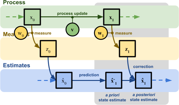
As anticipated in the previous part of this tutorial, the Kalman filter works in two steps: prediction and correction. The prediction step answers this question: given our current understand of the world (represented by $\hat{x}_0$ and $P_0$ ), how do we expect the system to evolve, solely based on our model? If we take into consideration our new model (9), we still expect no changes (on average) from $\hat{x}_0$ to $\hat{x}_1$ . However, we do expect $P_1$ to change, as now the variance of $\hat{x}_0$ increases steadily by $Q$ after each step. The introduction of the process noise indicates that we cannot blindly trust our model anymore. Updating the value of $P_0$ by adding $Q$ at each step stops the vanishing of $P_1$ , forcing the filter to doubt its own result.

(12) $\begin{equation*}\begin{align}P_1^{-} & \overset{\triangle}{=} P_0 +Q & &\\k_1 & = \frac{P_0 +Q}{P_0+R} & =& \frac{P_1^{-}}{P_0+R} \\P_1 & = \left(1-k_1\right) \left(P_0 +Q\right) &= &\left(1-k_1\right) P_1^{-}\end{align}\end{equation*}$

The quantity $P_0 + Q$ is sometimes referred to as $P_1^{-}$ , or a priori variance. The term a priori indicates that $P_1^{-}$ represents a belief on how $P_0$ should have evolved according to the model, before taking into consideration any sensor data. Once the measurement $z_1$ is integrated, $P_1^{-}$ turns into the a posteriori variance $P_1$ , which was derived previously.

$Q$	0.001
$R$	0.08

This change alone is not fixing all of our issues. But the resulting filter, above, is now responding correctly and its variance doesn’t vanish, as seen in the chart above.

Unfortunately, there is a trade-off between responsiveness and noise reduction. A filter that is very responsive will also be more susceptible to noise; a filter that can reduce most of the noise will take longer to respond to changes.

Model Prediction

Despite the introduction of the a priori variance $P_1^{-}$ , it is obvious that the filter is still reacting with a significant delay. This is because the value used for $Q$ is too low, causing the filter not to trust rapid changes in the temperature value.

If you do not know anything about the dynamic of the system, this is your best guess and the only thing you can do is tweaking the values of $Q$ and $R$ . There are cases in which some knowledge of the system is available. Generally speaking, equation (9) can be rewritten to include an arbitrary function $f\left(\cdot\right)$ that, taken the state of the system $x_0$ , indicates how it should evolve in the next time step, $x_1$ :

(13) $\begin{equation*} x_1 = f\left(x_0\right) + v\end{equation*}$

The equations that are derived from this formulation lead to the so-called extended Kalman filter (or EKF), which works for functions that are not necessarily linear. We will explore how it works in the fourth instalment of this tutorial: The Extended Kalman Filter.

❓ Why f(•) has to be linear?

The “magic” of the Kalman lies in a simple idea: both the sensor measurements and the best estimate so far follow a normal distribution, and the joint probability of two normal distributions remains a normal distribution.

This means that in the next time frame the process can be repeated, since the new best estimated is once again a normal distribution.

However, updating the model alters its probability distribution. Allowing any function can break the assumption of its normal distribution. And if that fails, the guarantee of optimality fails as well.

The reason why this does not happen when using a linear model is that a linear combination of two normal distribution is a normal distribution itself.

Extended Kalman filters are able to replace this linear constraints with a more relaxed one: the function has to be at least differentiable. What the filter does is then finding a linear approximation of the function around its current estimate. So, in a way, even EKFs are still relying on a linear model.

When the function is highly non-linear, even EFK can have issues adapting to its temperamental behaviour. In that case, another variant called the Unscented Kalman filter (UKF) finds ample application.

In order to simplify our derivation, we need to restrict our problem by imposing a constraint of linearity on $f$ . This means that the function $f$ can be expressed in terms of a product and a sum:

(14) $\begin{equation*} x_1 = A~x_0 + B + v\end{equation*}$

One can be tempted to simply state that:

(15) $\begin{equation*} \hat{x}_1 = A~\hat{x}_0 + B + v\end{equation*}$

but that would not be entirely correct. This is because what we have here is a probabilistic model. And so, the best way to extend the prediction step to include the a priori prediction for the evolution of $\hat{x}_0$ would be calculating its expected value:

(16) $\begin{equation*}\begin{align}\hat{x}_1^{-} &\overset{\triangle}{=} \mathrm{E} \left[\hat{x}_1\right] &=\\& = \mathrm{E} \left[A~\hat{x}_0 + B + v\right] &=\\& = \mathrm{E} \left[A~\hat{x}_0\right] + \mathrm{E} \left[B\right] + \mathrm{E} \left[v\right] &=\\& = A ~\mathrm{E} \left[\hat{x}_0\right] + B + 0 &=\\& = A ~\hat{x}_0 + B\end{align}\end{equation*}$

This new quantity, $\hat{x}_1^{-}$ , represents how we believe the system should evolve, if at the previous time step our estimated position was $\hat{x}_0$ . In the scientific literature it is known as the a priori state estimate, as it happens before (a priori) the measurement.

To complete the derivation, we also need to update our a priori prediction for $P_1^{-}$ . We can derive its exact value by calculating the variance of $\hat{x}_1$ :

(17) $\begin{equation*}\begin{align}P_1^{-} &\overset{\triangle}{=} \mathrm{Var} \left[ \hat{x}_1^{-}\right] &=\\& = \mathrm{Var} \left[ A~\hat{x}_0 + B + v \right] &= \\& = \mathrm{Var} \left[ A~\hat{x}_0\right] + \mathrm{Var} \left[B\right] + \mathrm{Var} \left[v \right] &= \\& = \mathrm{Var} \left[ A~\hat{x}_0 \right] + 0 + Q&= \\& = A^2 ~ \mathrm{Var} \left[\hat{x}_0 \right] + Q&= \\& = A^2 ~ P_0 + Q\end{align}\end{equation*}$

Adding a constant to a random variable does not change its variance, so $B$ bears no influence on the calculation. The last two steps are justified by the fact that:

(18) $\begin{equation*}$\mathrm{Var} \left[ A~X \right] = A^2 ~ \mathrm{Var} \left[X\right]$\end{equation*}$

In the scientific literature, $P_1^{-}$ is often expressed as $A~ P_0 ~ A + Q$ . This is because such a notation is more amenable to be expressed in a matrix form than $A^2 ~ P_0 + Q$ .

So, to recap:

(19) $\begin{equation*}\begin{align}\hat{x}_1^{-} & = A~\hat{x}_0 + B \\P_1^{-} & = A^2~P_0 +Q\end{align}\end{equation*}$

This leads to a more precise version of the Kalman filter that is able to take into account the evolution of the system. You can try this yourself using the interactive chart below:

$Q$	0.001
$R$	0.08

Compared to the original one, this time the filter is able to correctly re-adjust to the signal change. Setting $Q$ to $0$ will cause the filter to behave exactly like the first one presented at the beginning of the article.

It is important to remember that the version of the Kalman filter that has been derived so far is only able to integrate linear models. In a nutshell, this means that our filters are optimised to work with signals that are essentially straight lines. This is a strong limitations which will be revised in the following article.

❗ A different interperation for the process noise

The process noise is usually presented as the inherent unreliability of the system that we want to model. However, that is not the only way in which it can be conceptualised.

In fact, there are two scenarios which—from a mathematical point of view—will yield exactly the same results:

A nosy process, perfectly modelled by the filter
A perfect process, modelled imperfectly by the filter

In the former, the noise comes from the fact that the process in inaccurate (i.e.: the laws of motion are perfectly known, but the train moves unreliably). In the latter, the uncertainty is not injected in the system in the form of noise, but as a modelling error:

Realistically, both sources of noise are present. But what makes Statistics to powerful is that uncertainty due to lack of knowledge, errors and “true” randomness can all be modelled using the same mathematical tools.

Conclusion

In this article we completed the derivation of the Kalman filter, a popular statistical technique used for sensor de-noising and sensor fusion. Below you can see a diagram showing the most complex model build:

This includes a prediction of how the system is going to evolve over time, as long as a correction step which integrates readings from a sensor to reach to a better estimate.

You can play with a Kalman filter yourself using the interactive chart below:

$Q$	0.02
$R$	0.08

hghghg

Initialisation

$\begin{equation*}\begin{align*}\hat{x}_0 & & \textup{initial state} \\P_0 &= 1& \textup{initial variance} \\Q & & \textup{process noise variance} \\R & & \textup{measurement noise variance} \\A & & \textup{model coefficient} \\B & & \textup{model offset}\end{align}\end{equation}$

Prediction step
How we think the system should evolve, solely based on its model.

$\begin{equation*}\begin{align*}\hat{x}_1^{-} & = A~\hat{x}_0 + B & \textup{state prediction} \\P_1^{-} & = A^2 ~ P_0 +Q & \textup{variance prediction} \\\end{align}\end{equation}$

Correction step
The most likely estimation of the system state, integrating the sensor data.

$\begin{equation*}\begin{align*}k_1 & = \frac{P_1^{-}}{P_0+R} & \textup{Kalman gain} \\\hat{x}_1 &= \hat{x}_1^{-} \left(1-k_1\right) + z_1 \, k_1 & \textup{state update} \\P_1 & = \left(1-k_1\right) P_1^{-} & \textup{variance update}\end{align}\end{equation}$