The Mathematics of Epidemics

This online course introduces the topic of modelling and simulating epidemics. If you are interested in understanding how Mathematicians, Programmers and Data Scientists are studying and fighting the spread of diseases, this series of posts is what you are looking for.

Part 1. The Mathematics of Epidemics
Part 2. Simulating Epidemics
Part 3. From an Outbreak to an Epidemic

This online course is inspired by the recent COVID-19 pandemic. Now more than ever we need skilled and passionate people to focus on the complex subject of Epidemiology. I hope these articles will help some of you to get started.

All the revenue made from this article through Patreon will be donated to the National Emergencies Trust (NET) to help those most affected by the recent coronavirus outbreak. If you have recently become a patron for this reason, get in touch and I will add your contribution.

Become a Patron!

Introduction

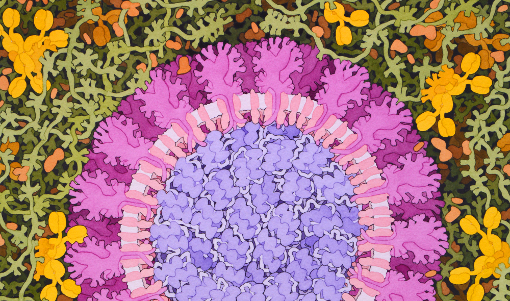
It is impossible to deny that the recent pandemics of COVID-19 has changed the world we live in. With a significant part of the world population under lockdown, most people living in Western countries have been—one way or another—affected by the novel coronavirus (below, an artistic rendering by David S. Goodsell). Now more than ever, we are bombarded with a constant stream of contradicting news and inconsistent policies. Technical terms such as exponential growth, social distancing and logarithmic plots are now commonly used on both TV and social media. And without the right background, it might be very difficult to make sense of the numbers that are constantly been updated every hour. When colleagues, friends and relatives are getting ill, it is only natural wanting to do everything in our power to help them. And, paradoxically, we are being told to stay home and do nothing. It is hard to understand how any good could actually come out of inaction.

As a Science Communicator—one which family has been affected—I feel is important I take this opportunity to add my contribution to the current discourse. Not the one surrounding COVID-19 (for which I am not really qualified to talk about), but the study and simulation of epidemics. Since 2015, I have talked extensively about the power of simulations, and how they could be used to solve a variety of different problem. From simulating the process of evolution by natural selection (Evolutionary Computation) to harnessing the power of modern GPUs (How to Use Shaders for Simulations), up to the creating photorealistic rendering of a planet’s sky (Volumetric Atmospheric Scattering).

If you want to understand how scientists model and simulate the evolution of epidemics and the spread of diseases on large populations, this is the right place. I sincerely hope this series of articles will not only give you the tools to better understand the terminology and numbers surrounding the current pandemics. I ultimately hope it will inspire more passionate developers to proactive study and research the fascinating fields of epidemiology. Just a few days ago, the Royal Society started coordinating the Rapid Assistance in Modelling the Pandemic (RAMP): an urgent call to action addressed to the scientific modelling community, recruiting developers, programmers and data scientists all over the UK to study and predict the evolution of the current COVID-19 pandemic. While hundreds of thousands nurses and doctors are saving lives every day, there are probably as many researchers and developers who are working around the clock to end the current pandemic. Those are hidden heroes which might end up saving your life, even though you never met them.

There are probably many researchers and developers who are working around the clock to end the current pandemic. Those are hidden heroes which might end up saving your life, even though you never met them.

Modelling Epidemics

Epidemics are very complex social phenomena that involve millions of people, over hundreds of countries. They are undeniably driven by the individual choices of each person involved, although they ultimately follow very recognisable patterns.

At first glance, this might seem counterintuitive. If the decisions of each person are arbitrary and unpredictable, how could an overall population made out of millions of them become suddenly predictable?

Let’s try to answer this question with a simple example. Let’s imagine a population of arrows, each one pointing in a different direction (below). What is the “overall” direction they point at? If we assume there is a sufficiently large number of them, it is also reasonable to assume that for each arrow pointing in a certain direction, there is another one pointing in the opposite one. The more arrows we have, the more confident we can be about the fact that their sum cancels out.

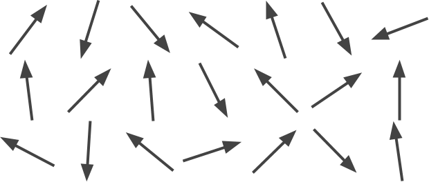
This concept is related to the Law of Large Numbers, which describes the overall behaviour of large numbers of random phenomena. Even if we assumed human behaviour to be completely random (which is not), we would still be able to model the overall behaviour of a sufficiently large population. So, we do not need to take into account the behaviour of each individual person to draw meaningful conclusions on the overall population.

Exponential Growth

One of the most simple ways to model the evolution of an epidemic is to only focus on the number of infected people, $X$ , and how it varies over time. In an ideal scenario, we can imagine one single person infecting a certain number of people during their lifetime, $r$ . For instance, if $r=2$ it means that each person will infect two more. And those two, will infect two more each. We can express this mathematically by saying that the number of people infected doubles each day:

(1) $\begin{equation*} X\left(t+1\right)=r X\left(t\right) \end{equation*}$

In the expression above, $X\left(t\right)$ represents the number of infected people on a certain day $t$ , while $X\left(t+1\right)$ the ones infected on the following day. That is known as a recurrence relationship, as the value for $t+1$ is defined in terms of the value for $t$ . If you are familiar with programming, recurrence relationships are the mathematical equivalent of recursive functions.

We can expand the equation by noticing that it follows a simple pattern:

(2) $\begin{equation*} \begin{align} X\left(0\right)&=& 1 & & &=&{r}^0\\ X\left(1\right)&=& r X\left(0\right) &=& r &=&{r}^1\\ X\left(2\right)&=& r X\left(1\right) &=& r r &=&{r}^2\\ X\left(3\right)&=& r X\left(2\right) &=& r {r}^2 &=&{r}^3 \end{align} \end{equation*}$

It is easy to see that we can generalise this with a traditional closed-form expression:

(3) $\begin{equation*} X\left(t\right)={r}^t \end{equation*}$

which is an exponential curve. This means that if every infected person always infects $r$ other people, the epidemics follows an exponential growth.

$r$

1.5

📚 The Malthusian growth model

Equation (3) is a special case of the slightly more complex Malthusian growth model:

(4) $\begin{equation*} X\left(t\right)=X\left(0\right) \exp \left\{rt\right\} \end{equation*}$

where $X\left(0\right)$ represents the initial population.

The equation was firstly derived by Thomas Robert Malthus in 1798, where it was used to described the growth of a population over time.

Logistic Growth

The model presented in the section above works very well during the early stages of an epidemic. However, it is clear that such growth cannot be sustained because we will reach the point where all people are infected. After an initial explosion, the number of infected people will start growing slower because the more people are infected, the harder it is to find someone new who can be infected.

The idea is to change (3) by adding a factor that can slow down the exponential growth. We can think about $r$ not as a constant anymore, but as a function which depends on how many people have already been infected, $X\left(t\right)$ .

When the model starts, $r$ should have a base value $r_0$ , which will cause the exponential growth seen in the previous section. However, the more we approach a certain capacity $C$ , the harder it is to infect people, and the smaller $r\left(X\left(t \right)\right)$ becomes.

What we want, in a nutshell, is to enforce the following properties:

(5) $\begin{equation*} \begin{align} X\left(t\right) = 0 &\rightarrow & r =r_0 \\ X\left(t\right) = C &\rightarrow & r = 0 \end{align} \end{equation*}$

The simplest way to model this new function is with a linear mapping:

(6) $\begin{equation*} r = r_0\left(1 - \frac{X\left(t \right)}{C}\right) \end{equation*}$

We can now update (1), replacing $r$ with (6):

(7) $\begin{equation*} \begin{align} X\left(t+1\right)&=&\boxed{r} X\left(t\right) \\ X\left(t+1\right)&=&\boxed{r_0\left(1 - \frac{X\left(t \right)}{C}\right)}X\left(t \right) \end{align} \end{equation*}$

The new equation results in the so-called logistic growth, which approximately very well the growth of populations and the spread of diseases.

Converting the recurring expression for $X\left(t\right)$ into a closed-form one is not as easy as it was for the exponential growth, as this is now a fully-fledged ordinary differential equation. For this reason, I will omit the full derivation; its solution take the form of the well-known logistic function:

(8) $\begin{equation*} X\left(t\right) = \frac{C}{1+\left( \frac{C-X\left(0\right)}{X\left(0\right)} \right) \exp\left\{-r_0 t\right\} } \end{equation*}$

where:

$t$ : the time after the first infection (for instance, the number of days);
$X\left(t\right)$ : the infected population at time $t$ ;
$X\left(0\right)$ : the number of infected people at time $t=0$ ;
$C$ : the number of infected people after which no new infections are possible (known as the carrying capacity);
$r_0$ : how many other people, on average, each infected person infects (known as the basic reproduction number).

$r_0$	1.5
$X\left(0\right)$	0.01

📚 Ordinary Differential Equations

Differential equations are a way of expressing how a function $X\left(t\right)$ changes. While “traditional” equations give an expression to calculate $X\left(t\right)$ as a function of $t$ , differential equations express how the rate of change of $X$ evolves, based on its current value.

For instance, if the variable $X\left(t\right)$ never changes its value, its rate of change will be zero:

(9) $\begin{equation*} \frac{\partial X}{\partial t} = 0 \end{equation*}$

This expression only tells that the function never changes, but does not tell what value it actually has. For instance, in the case of an exponential growth, the rate at which $X$ grows depends on the value of $X$ itself:

(10) $\begin{equation*} \frac{\partial X}{\partial t} = r X \end{equation*}$

Some phenomena, especially in Physics, are better described by differential equations.

Solving a differential equations means finding the value of $X\left(t\right)$ . It is not always possible to find a closed-form expression that represents for $X\left(t\right)$ , given a differential equation. However, it is often possible to find an approximated solution using numerical methods (such as the Runge–Kutta methods).

Compartmental Models

Both the exponential and logistic growth can be applied to a variety of different scenarios, some of which are not related to the study of epidemics. In fact, they were originally designed to model the growth of a generic population.

In the scientific literature, there are several mathematical models that have been created specifically for the study of how diseases spread in a given population. A branch of them models are called compartmental models, as they divide the general population into different groups called or compartments (and assuming no new people are born or can enter into the system).

One of the most simple compartmental models is called SIR, from the initials of the three groups it models: susceptible, infected and recovered people. The idea is that, at time $t=0$ , all people are susceptible to an infection. Among people in this group, a given infection can spread following an exponential growth. The infection can lead to two outcomes: recovery or death. In both cases, a person cannot contract the infection twice; in one case because they gain immunity, in another because they are dead. This is why this group is referred to as removed: because they do not play a role anymore to the spread of the disease. Resistant is another term that is often seen in the literature. The model was originally developed by William Ogilvy Kermack and Anderson Gray McKendrick in 1927, but gained popularity only in 1979.

The SIR model is often indicated using the following notation, which explains the journey of a person from the different compartments:

(11) $\begin{equation*} \mathcal{S} \rightarrow \mathcal{I} \rightarrow \mathcal{R} \end{equation*}$

The purpose of a SIR model is to find a series of equations to calculate, at a specific time $t$ , how many people are in each compartment. So, a SIR model aims to find a definition for $S\left(t\right)$ , $I\left(t\right)$ and $R\left(t\right)$ .

They are best defined as a series of differential equations:

(12) $\begin{equation*} \begin{align} \frac{\partial S}{\partial t} &= -\beta \frac{SI}{N} & \\ \frac{\partial I}{\partial t} &= +\beta \frac{SI}{N} & -\gamma I \\ \frac{\partial R}{\partial t} &= &+\gamma I \\ \end{align} \end{equation*}$

(13) $\begin{equation*} \begin{align} N &= S+I+R \\ \end{align} \end{equation*}$

where:

$\beta$ : controls how often an interaction between a susceptible and infected people results in a new infection;
$\gamma$ : the rate at which infected people recover (or die) and move into the removed compartment.

If we want to be more precise, we can also indicate on the arrows the parameters that control the flow between different compartments:

(14) $\begin{equation*} \mathcal{S} \xrightarrow{\beta SI} \mathcal{I} \xrightarrow{\gamma I} \mathcal{R} \end{equation*}$

In this model, $r_0 =\frac{\beta}{\gamma}$ .

Below, you can find an interactive tool to simulate the evolution of a SIR model. It is based directly on the differential equations presented in (12).

$\beta$	0.6
$\gamma$	0.1
$I_0$	1

The chart above uses Hans Nesse‘s implementation of the Runge-Kutta method.

Other Models

There are several other models available, which include different compartments. A simpler one is the SIS model, which includes the possibility for people of being reinfected.

(15) $\begin{equation*} \mathcal{S} \rightarrow \mathcal{I} \rightarrow \mathcal{S} \end{equation*}$

A more complex one, SEIRS, contemplates the possibility who have been exposed to the disease but are not infectious yet. This compartment is referred to as exposed:

(16) $\begin{equation*} \mathcal{S} \rightarrow \mathcal{E} \rightarrow \mathcal{I} \rightarrow \mathcal{R} \rightarrow \mathcal{S} \end{equation*}$

What’s Next…

The first article in this online course about epidemics explored how Mathematicians and Data Scientists model them using differential equations. The exponential and logistic growth curves were introduced, followed by the compartmental models. Among the latter, the SIR model is one of the most popular.

The next article, Simulating Epidemics, will move away from the mathematical formulation of epidemics, to focus on a more programmatical and flexible approach.

Part 1. The Mathematics of Epidemics
Part 2. Simulating Epidemics
Part 3. From an Outbreak to an Epidemic

Additional Resources

Download

Become a Patron!
You can download the Unity package presented in this tutorial on Patreon. The package contains all the scripts, scenes, prefabs and sprites necessary to recreate the images presented in this online series, including the one below.

All of the revenue from this tutorial will be donated to the National Emergencies Trust (NET), to help those most affected by the recent coronavirus outbreak.

💖 Support this blog

This website exists thanks to the contribution of patrons on Patreon. If you think these posts have either helped or inspired you, please consider supporting this blog.

Follow @AlanZucconi

📧 Stay updated

You will be notified when a new tutorial is released!

📝 Licensing

You are free to use, adapt and build upon this tutorial for your own projects (even commercially) as long as you credit me.

You are not allowed to redistribute the content of this tutorial on other platforms, especially the parts that are only available on Patreon.

If the knowledge you have gained had a significant impact on your project, a mention in the credit would be very appreciated. ❤️🧔🏻

Tony Brine

May 25, 2020

Firstly, many thanks for posting this. So easy to follow, so interesting, so relevant.
Just one question. In the SIR model, shouldn’t the green shaded curve be the “infected” curve (rise followed by fall)?

Reply to Tony
- Alan Zucconi
  
  May 29, 2020
  
  You’re right!
  Thank you for spotting that, I have now corrected the labels!
  
  Reply to Alan
Izem Kenyatta

December 14, 2023

Hey, thanks for this helpful information. I just had 1 remark. The link you put here (The chart above uses Hans Nesse‘s implementation of the Runge-Kutta method.) isn’t accessible anymore and I can’t find it anywhere else. Could you help me out real quick, thank you

Reply to Izem

Webmentions

From an Outbreak to an Epidemic - Alan Zucconi December 14, 2023

[…] Part 1. The Mathematics of Epidemics […]

Simulating Epidemics - Alan Zucconi December 14, 2023

Published

March 30, 2020

Alan Zucconi in Discussion, Maths, Tutorial | March 30, 2020