
This tutorial will introduce the Transformation Matrix, one of the standard technique to translate, rotate and scale 2D graphics. The first part of this series, A Gentle Primer on 2D Rotations, explaines some of the Maths that is be used here.
- Introduction
- Part 1. Matrix notation
- Part 2. Adding translations
- Part 3. Composition
- Part 4. Inversion
- Part 5. Rotation around a point
- Conclusion
Introduction
In the previous post we have seen how a 2D point  can be represented in the plane, and how trigonometry links its Polar and Cartesian representations:
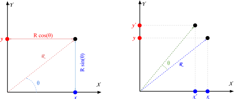
In a nutshell:
![\[x=R \, \cos\left(\theta\right ) \]](https://www.alanzucconi.com/wp-content/ql-cache/quicklatex.com-e8b2e786f6267b518d76c162e95cad2a_l3.png "Rendered by QuickLaTeX.com")
![\[y=R \, \sin\left(\theta\right ) \]](https://www.alanzucconi.com/wp-content/ql-cache/quicklatex.com-6aefa2309257048436b8d20d744271fe_l3.png "Rendered by QuickLaTeX.com")
The second important result is that any given point an be rotated by an angle  around the origin as follow:
![\[{x}' = x \, \cos\left(\theta\right)- y\, \sin\left(\theta\right)\]](https://www.alanzucconi.com/wp-content/ql-cache/quicklatex.com-5fade6d9535a96a1ce3e8729b8019470_l3.png "Rendered by QuickLaTeX.com")
![\[{y}' = x\, \sin\left(\theta\right) + y \, \cos\left(\theta\right)\]](https://www.alanzucconi.com/wp-content/ql-cache/quicklatex.com-b674791ad82cae94818ac9e2ff6c17b7_l3.png "Rendered by QuickLaTeX.com")
These are the only two notions you need to understand this tutorial.
Matrix notation
When it comes to 3D graphics, there’s an alternative representation that is often encountered. A rotation can, in fact, be expressed as a matrix multiplication. To do this, let’s express as the column vector  . The problem is now finding a matrix
  so that:
![\[T\left(\theta\right)\cdot\begin{bmatrix}x \\ y\end{bmatrix}=\begin{bmatrix}x\,\cos\left(\theta\right) -y\,\sin\left(\theta\right) \\x\,\sin\left(\theta\right) + y\,\cos\left(\theta\right)\end{bmatrix}=\begin{bmatrix}{x}' \\ {y}'\end{bmatrix}\]](https://www.alanzucconi.com/wp-content/ql-cache/quicklatex.com-c25c5e3d4576756c172e415c20e9f5cc_l3.png "Rendered by QuickLaTeX.com")
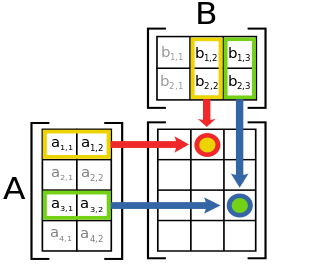
❓ Matrix Multiplication
Remembering matrix multiplication:
![\[\begin{bmatrix}a & b \c & d\end{bmatrix}\cdot\begin{bmatrix}x \ y\end{bmatrix}=\begin{bmatrix}x a + yb \xc + yd\end{bmatrix}\]](https://www.alanzucconi.com/wp-content/ql-cache/quicklatex.com-84e54e10dcf3ec46907b53e7963914c5_l3.png "Rendered by QuickLaTeX.com")
Please, note that the result is a vector with one column. This makes sense, because the result is another point in the 2D plane.
The matrix can be defined as:
![\[\underbrace{\begin{bmatrix}\cos\left(\theta\right) & -\sin\left(\theta\right) \\\sin\left(\theta\right) & \cos\left(\theta\right)\end{bmatrix}}_{T\left(\theta\right)}\cdot\begin{bmatrix}x \\ y\end{bmatrix}=\begin{bmatrix}x\,\cos\left(\theta\right) -y\,\sin\left(\theta\right) \\x\,\sin\left(\theta\right) + y\,\cos\left(\theta\right)\end{bmatrix}=\begin{bmatrix}{x}' \\ {y}'\end{bmatrix}\]](https://www.alanzucconi.com/wp-content/ql-cache/quicklatex.com-daad9536a552b3e92cbf54b3e7643e4b_l3.png "Rendered by QuickLaTeX.com")
Every rotation of radians in the 2D plane can be obtained by multiplying a column vector by .
Adding translations
There are other operations which, unfortunately, cannot be achieved with this matrix. Translations is one of them. What we want is a new matrix  such that:
![\[T\left(t_x, t_y\right)\cdot\begin{bmatrix}x \\ y\end{bmatrix}=\begin{bmatrix}x+ t_x \\y+ t_y\end{bmatrix}\]](https://www.alanzucconi.com/wp-content/ql-cache/quicklatex.com-295f027d1d1a5b65d3cd31b1f04f3ebd_l3.png "Rendered by QuickLaTeX.com")
This is not possible with the current setting. In order to obtain this result, we need to modify the way is represented.
![\[\underbrace{\begin{bmatrix}1&0 & t_x \\0 & 1 & t_y \\0 & 0 & 1 \\\end{bmatrix}}_{T\left(t_x, t_y\right)}\cdot\begin{bmatrix}x \\ y \\ 1\end{bmatrix}=\begin{bmatrix}x+t_x\\y +t_y \\ 1\end{bmatrix}\]](https://www.alanzucconi.com/wp-content/ql-cache/quicklatex.com-7ebc1704849fd24e68971e0d2fdd3e5e_l3.png "Rendered by QuickLaTeX.com")
The point is now represented by the three dimensional column vector  . This is necessary in order to make the matrix multiplication works, since the new
  now has three rows and columns.
❓ The Transformation Matrix
This technique is currently being used in most 2D graphics framework. The matrix is often called the Transformation matrix and can be used to perform the following operations:
Composition
Using matrices to perform transformation has an incredible advantage: they can be multiplied together to perform multiple transformation. A single matrix can hold as many transformation as you like. In a nutshell:
![\[T_2 \cdot\left (T_1 \cdot\begin{bmatrix}x \\ y \\ 1\end{bmatrix}\right)=\left (T_2 \cdot T_1\right)\cdot\begin{bmatrix}x \\ y \\ 1\end{bmatrix}\]](https://www.alanzucconi.com/wp-content/ql-cache/quicklatex.com-f9f0ad177726e4b8c5b6cb48948eb005_l3.png "Rendered by QuickLaTeX.com")
This is true because matrix multiplication is an associative operator. It is important to remember, however, that these transformations are not commutative. This means that  is not the same as
  . Intuitively, this is obvious: rotating and translating is different from translating and then rotation.
Inversion
Transformations can be undone. For every transformation matrix which does rotates or translates, there is a matrix  which performs the “opposite” operation. This means that if we apply , followed by , we obtain the original point:
![\[T^{-1} \cdot\left (T \cdot\begin{bmatrix}x \\ y \\ 1\end{bmatrix}\right)=\begin{bmatrix}x \\ y \\ 1\end{bmatrix}\]](https://www.alanzucconi.com/wp-content/ql-cache/quicklatex.com-1b8866aa3b95df8de74fb5da6bd3c5af_l3.png "Rendered by QuickLaTeX.com")
By using the associative property, we can get a glimpse of what this matrix is:
![\[\left (T^{-1} \cdotT\right)\cdot\begin{bmatrix}x \\ y \\ 1\end{bmatrix}=\begin{bmatrix}x \\ y \\ 1\end{bmatrix}\]](https://www.alanzucconi.com/wp-content/ql-cache/quicklatex.com-080c2c62e1f111700d2469a447aaf2c0_l3.png "Rendered by QuickLaTeX.com")
![\[\left (T^{-1} \cdotT\right)\cdot\begin{bmatrix}x \\ y \\ 1\end{bmatrix}=\mathbb{I}\cdot\begin{bmatrix}x \\ y \\ 1\end{bmatrix}\]](https://www.alanzucconi.com/wp-content/ql-cache/quicklatex.com-c7a6c2e50f9fda2cbdd4c85d73afb12e_l3.png "Rendered by QuickLaTeX.com")
![\[T^{-1} \cdot T = \mathbb{I}\]](https://www.alanzucconi.com/wp-content/ql-cache/quicklatex.com-28b14aa4d31bf91da69d005631a27883_l3.png "Rendered by QuickLaTeX.com")
If you have a basic knowledge of matrix algebra, you should recognise this: is the inverse matrix of . Inverting a matrix is a non trivial task, and goes beyond the scope of this tutorial. However, you don’t really need to know how to invert a matrix to undo a transformation. Because of the way the transformation matrix has been constructed, it is always true that:
![\[T\left(-\theta\right) \cdot\left (T\left(+\theta\right)\cdot\begin{bmatrix}x \\ y \\ 1\end{bmatrix}\right)=\begin{bmatrix}x \\ y \\ 1\end{bmatrix}\]](https://www.alanzucconi.com/wp-content/ql-cache/quicklatex.com-43e83b62c926b22b7707692d7ed598e9_l3.png "Rendered by QuickLaTeX.com")
![\[T\left(-x,-y\right) \cdot\left (T\left(+x,+y\right)\cdot\begin{bmatrix}x \\ y \\ 1\end{bmatrix}\right)=\begin{bmatrix}x \\ y \\ 1\end{bmatrix}\]](https://www.alanzucconi.com/wp-content/ql-cache/quicklatex.com-8f55f4d1dea4abbe44c26ad1fddc7fe4_l3.png "Rendered by QuickLaTeX.com")
The meaning of these two equations should be intuitive to grasp: if you rotate a point of angles, followed by a rotation of  , you get the original point. The same applies for translations.
![\[T\left(+\theta\right)^{-1} = T\left(-\theta\right)\]](https://www.alanzucconi.com/wp-content/ql-cache/quicklatex.com-64c3702fea6368556b3dde40e33a92a3_l3.png "Rendered by QuickLaTeX.com")
![\[T\left(+x,+y\right)^{-1} = T\left(-x,-y\right)\]](https://www.alanzucconi.com/wp-content/ql-cache/quicklatex.com-665ce71150113626c48c3eec715836f0_l3.png "Rendered by QuickLaTeX.com")
From this, it follows that if you have a series of elementary rotations and translations, the inverse of their composition is the composition of their inverses, in reversed order:
![\[\left( T_n \cdot T_{n-1}\cdot \dots \cdot T_2\cdot T_1 \right)^{-1}= T_1^{-1} \cdot T_2^{-1} \cdot T_{n-1}^{-1}\cdot \dots \cdot T_n^{-1}\]](https://www.alanzucconi.com/wp-content/ql-cache/quicklatex.com-a08b3e2e3d088596030e6f8ffd2a67d6_l3.png "Rendered by QuickLaTeX.com")
❓ Singular Matrix
From a more general point of view, it is not true that all transformations can be undone. For instance the following transformations cannot be undone:
![\[\begin{bmatrix}0 & 0 & 0 \\0 & 1 & 0 \\0 & 0 & 1\end{bmatrix}\cdot\begin{bmatrix}x \\ y \\ 1\end{bmatrix}\right)=\begin{bmatrix}0 \\ y \\ 1\end{bmatrix}\right)\]](https://www.alanzucconi.com/wp-content/ql-cache/quicklatex.com-6c314b0ea79f581a440a0be92326aedf_l3.png "Rendered by QuickLaTeX.com")
Multiplying the
 component by zero destroys its information, which cannot be restored with another multiplication. Such transformation, however, is neither a rotation nor a translation. In this particular case, the matrix cannot be inverted. When this occurs, it is also referred as singular or degenerate. A matrix is singular is and only if its determinant is zero.
Rotation around a point
As seen in the previous part of this tutorial (A Gentle Primer on 2D Rotations), to rotate around an arbitrary point, we need to first make that our new origin of the Cartesian plane. Then we rotate the point, and finally we restore the origin of the plane. This can be expressed a composition of three transformations:
![\[T\left(P_x,P_y\right) \cdot T\left(\theta\right) \cdot T\left(-P_x,-P_y\right)\]](https://www.alanzucconi.com/wp-content/ql-cache/quicklatex.com-7af36dbba5425d88a4adb8b144d89b0b_l3.png "Rendered by QuickLaTeX.com")
It’s important to remember that, despite the order in which they are written, the first transformation is the one on right.


Conclusion
This post has introduced the transformation matrix, which is one of the standard ways in which transformations are stored and performed in computer graphics. We have explored the following transformations:
- Translation by
 :
:
![\[\underbrace{\begin{bmatrix}1 & 0 & t_x\\0 & 1 & t_y \\0 & 0 & 1\end{bmatrix}}_{T\left(t_x, t_y\right)}\cdot\begin{bmatrix}x \\ y \\ 1\end{bmatrix}=\begin{bmatrix}x + t_x \\x + t_y \\1\end{bmatrix}\]](https://www.alanzucconi.com/wp-content/ql-cache/quicklatex.com-f05823bee9681077444892673444dcca_l3.png "Rendered by QuickLaTeX.com")
- Rotation by around the origin:
![\[\underbrace{\begin{bmatrix}\cos\left(\theta\right) & -\sin\left(\theta\right) & 0\\\sin\left(\theta\right) & \cos\left(\theta\right) & 0 \\0 & 0 & 1\end{bmatrix}}_{T\left(\theta\right)}\cdot\begin{bmatrix}x \\ y \\ 1\end{bmatrix}=\begin{bmatrix}x\,\cos\left(\theta\right) -y\,\sin\left(\theta\right) \\x\,\sin\left(\theta\right) + y\,\cos\left(\theta\right) \\1\end{bmatrix}\]](https://www.alanzucconi.com/wp-content/ql-cache/quicklatex.com-f473fc2c6b313c6644a3c16575d39704_l3.png "Rendered by QuickLaTeX.com")
- Rotation by around the point
 :
:
![\[T\left(P_x,P_y\right) \cdot T\left(\theta\right) \cdot T\left(-P_x,-P_y\right) \cdot \begin{bmatrix}x \\ y \\ 1\end{bmatrix}\]](https://www.alanzucconi.com/wp-content/ql-cache/quicklatex.com-69f6f1bc3421fea2eb2a2f42084dc94f_l3.png "Rendered by QuickLaTeX.com")
The main advantage of the matrix notation is that transformations can be composed by multiplying their respective transformation matrices. This also allows to “undo” transformation by calculating the inverse of its matrix.
The next post in this series will focus on the geometrical consequences of the equations we have derived. This will help to demystify one of the most misunderstood concept of Maths: complex numbers. Their understanding is essential for quaternions.
Other resources
- Part 1. A Gentle Primer on 2D Rotations
- Part 2. The Transformation Matrix
- Part 3. Rotations in the Complex Plane
- Part 4. Understanding Rotations in 3D
- Part 5. Understanding Quaternions
- Matrices aren’t scary. They’re essential.
Leave a Reply