
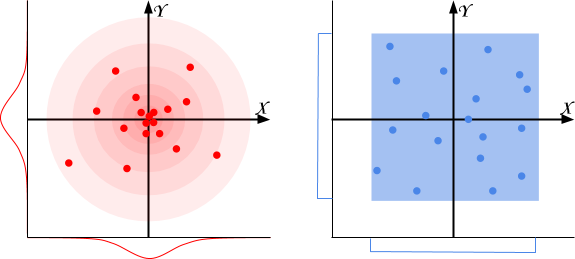
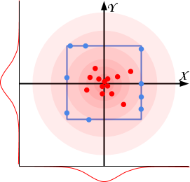
In a previous post I’ve introduced the Gaussian distribution and how it is commonly found in the vast majority of natural phenomenon. It can be used to dramatically improve some aspect of your game, such as procedural terrain generation, enemy health and attack power, etc. Despite being so ubiquitous, very few gaming frameworks offer functions to generate numbers which follow such distribution. Unity developers, for instance, heavily rely on Random.Range which generates uniformly distributed numbers (in blue). This post will show how to generate Gaussian distributed numbers (in red) in C#.
I’ll be explaining the Maths behind it, but there is no need to understand it to use the function correctly. You can download the RandomGaussian Unity script here.
Step 1: From Gaussian to uniform
Many gaming frameworks only include functions to generate continuous uniformly distributed numbers. In the case of Unity3D, for instance, we have Random.Range(min, max) which samples a random number from min and max. The problem is to create a Gaussian distributed variable out of a uniformly distributed one.
Sample two Gaussian distributed values
 Let’s imagine we already have two independent, normally distributed variables:
![\[X \sim \mathcal{N} \left(0,1 \right)\]](https://www.alanzucconi.com/wp-content/ql-cache/quicklatex.com-d284f3e30bc88400fb3b62afd4d9075a_l3.png "Rendered by QuickLaTeX.com")
![\[Y \sim \mathcal{N} \left(0,1\right)\]](https://www.alanzucconi.com/wp-content/ql-cache/quicklatex.com-bc3edb979a837391218d384403f9139f_l3.png "Rendered by QuickLaTeX.com")
from which we sampled two values,  and
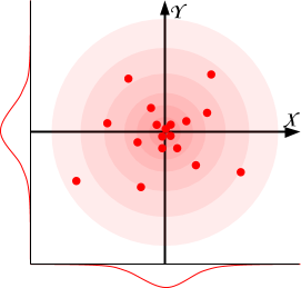
and  , respectively. Sampling several of these points in the Cartesian plane will generate a roundly shaped cloud centred at
  .
.
Calculate their joint probability
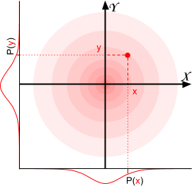 The probability of having a certain
  is defined as the probability sampling from
  , times the probability of sampling from
  . This is called joint probability and since samplings from and are independent from each other:
![\[P(x,y) = P(x)P(y) =\]](https://www.alanzucconi.com/wp-content/ql-cache/quicklatex.com-e133e0a946c8bad9e4adb4674d2f6a21_l3.png "Rendered by QuickLaTeX.com")
![\[ =\frac{1}{\sqrt{2\pi }}e^{-{\frac{x^2}{2}}}\frac{1}{\sqrt{2\pi }}e^{-{\frac{y^2}{2}}} =\frac{1}{2\pi}e^{-{\frac{x^2+y^2}{2}}}\]](https://www.alanzucconi.com/wp-content/ql-cache/quicklatex.com-955bf8c60e3f5718992b42557d50c407_l3.png "Rendered by QuickLaTeX.com")
Switch to polar coordinates
The point can be represented in the plane using polar coordinates, with an angle  and its distance from the origin
  :
:
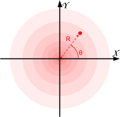
![\[R=\sqrt{x^2+y^2}\]](https://www.alanzucconi.com/wp-content/ql-cache/quicklatex.com-5a7cc40af5e54ad512d032c53e7a71f5_l3.png "Rendered by QuickLaTeX.com")
![\[\theta=arctan\left (\frac{y}{x}\right )\]](https://www.alanzucconi.com/wp-content/ql-cache/quicklatex.com-bb2086cd8f5e4520722aeac84a753dd1_l3.png "Rendered by QuickLaTeX.com")
Now the original point can be expressed as a function of and :
![\[x = R cos\left(\theta\right)\]](https://www.alanzucconi.com/wp-content/ql-cache/quicklatex.com-eeb2d380b7cb197da853971ecd257b2e_l3.png "Rendered by QuickLaTeX.com")
![\[y = R sin\left(\theta\right)\]](https://www.alanzucconi.com/wp-content/ql-cache/quicklatex.com-3bc8b8a5c8f6dc341cab2100160a49e0_l3.png "Rendered by QuickLaTeX.com")
Rewrite the joint probability
We can now rewrite the joint probability  :
:
![\[\frac{1}{2\pi }e^{-{\frac{x^2+y^2}{2}}}=\frac{1}{2\pi}e^{-{\frac{R^2}{2}}}=\left (\frac{1}{2\pi } \right )\left (e^{-{\frac{R^2}{2}}} \right )\]](https://www.alanzucconi.com/wp-content/ql-cache/quicklatex.com-aa81ab2577eeab0c6165e6ba55da2506_l3.png "Rendered by QuickLaTeX.com")
which is the product of the two probability distributions:
![\[R^2 \sim Exp\left(\frac{1}{2}\right)\]](https://www.alanzucconi.com/wp-content/ql-cache/quicklatex.com-70c85b963573f710d34e69efc0edfb8c_l3.png "Rendered by QuickLaTeX.com")
![\[\theta \sim Unif(0,2\pi) = 2\pi Unif(0,1)\]](https://www.alanzucconi.com/wp-content/ql-cache/quicklatex.com-5ad0166fedf6ab6e860843676033236a_l3.png "Rendered by QuickLaTeX.com")
Expanding the exponential distribution
While is already in a form which can be expressed using a uniformly distributed variable, a little bit more work is necessary for  . Remembering the definition of the exponential distribution:
![\[Exp(\lambda)=\frac{-log(Unif(0,1))}{\lambda}\]](https://www.alanzucconi.com/wp-content/ql-cache/quicklatex.com-8fb84c0fd163f9d8b9aef868c520237b_l3.png "Rendered by QuickLaTeX.com")
![\[R \sim \sqrt{-2log\left( Unif(0,1)\right)}\]](https://www.alanzucconi.com/wp-content/ql-cache/quicklatex.com-040455d3657ecd4eab573451c4e189a0_l3.png "Rendered by QuickLaTeX.com")
Now both and , which are coordinates of a point generated from two independent Gaussian distributions, can be expressed using two uniformly distributed values.
Step 2: From uniform to Gaussian
We can now reverse the procedure done in Step 1 to derive a simple algorithm:
- Generate two random numbers

- Use them to create the radius
 and the angle
- Convert
 from polar to Cartesian coordinates:
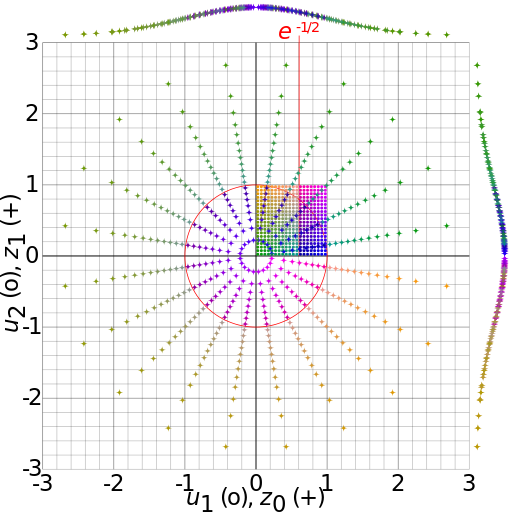
This is know as the Box-Muller transform. The image below (from Wikipedia) shows how the uniformly distributed points from the unit square are re-mapped by the Box-Muller transform onto the Cartesian plane, in a Gaussian fashion.
Step 3: The Marsaglia polar method
The Box-Muller transform has a problem: it uses trigonometric functions which are notoriously slow. To avoid that, a slightly different technique exists, called the Marsaglia polar method. Despite being similar, it stars from an uniformly distributed point in the interval  . This point must fit within the unit circle and shouldn’t be the origin ; if it doesn’t, another one has to be chosen.
public static float NextGaussian() {
    float v1, v2, s;
    do {
        v1 = 2.0f * Random.Range(0f,1f) - 1.0f;
        v2 = 2.0f * Random.Range(0f,1f) - 1.0f;
        s = v1 * v1 + v2 * v2;
    } while (s >= 1.0f || s == 0f);

    s = Mathf.Sqrt((-2.0f * Mathf.Log(s)) / s);

    return v1 * s;
}
Approximately 21% of the points will be rejected with this method.
Step 4: Mapping to arbitrary Gaussian curves
The algorithm described in Step 3 provides a way to sample from  . We can transform that into any arbitrary
  like this:
public static float NextGaussian(float mean, float standard_deviation)
{
    return mean + NextGaussian() * standard_deviation;
}
 There is yet another problem: Gaussian distributions have the nasty habit to generate numbers which can be quite far from the mean. However, clamping a Gaussian variable between a
 min and a max can have quite catastrophic results. The risk is to squash the left and right tails and having a rather bizarre function with three very likely values: the mean, the min and the max. The most common technique to avoid this is to take another sample if it falls outside its range:
public static float NextGaussian (float mean, float standard_deviation, float min, float max) {
	float x;
	do {
		x = NextGaussian(mean, standard_deviation);
	} while (x < min || x > max);
	retun x;
}
Another solution changes the parameter of the curve so that min and max are at 3.5 standard deviations from the mean (which should contain more than 99.9% of the sampled points).
Conclusion
This tutorial shows how to sample Gaussian distributed numbers starting from uniformly distributed ones. You can download the complete RandomGaussian script for Unity here.
Other resources
- Probability and Games: Damage Rolls: a very detailed explanation of how dices can be used to sample from different distributions;
- ProjectRhea: the principle of how to generate a Gaussian random variable;
- Sampling From the Normal Distribution: a similar tutorial;
- Box-Muller transforms: a more Maths-y tutorial.
- Part 1: Understanding the Gaussian distribution
- Part 2: How to generate Gaussian distributed numbers
💖 Support this blog
This website exists thanks to the contribution of patrons on Patreon. If you think these posts have either helped or inspired you, please consider supporting this blog.
📧 Stay updated
You will be notified when a new tutorial is released!
📝 Licensing
You are free to use, adapt and build upon this tutorial for your own projects (even commercially) as long as you credit me.
You are not allowed to redistribute the content of this tutorial on other platforms, especially the parts that are only available on Patreon.
If the knowledge you have gained had a significant impact on your project, a mention in the credit would be very appreciated. ❤️🧔🏻
Hey Alan,
I can’t download the unity code for this, it redirects me to patreon (where I already sponsor you) but there’s nothing there!
https://www.patreon.com/posts/3331323
Hey! That download is available for the $5+ patrons! 🙂
You’re such an asshole
Most things from Alan I read are of good and very good quality. I think it is fair to ask for some money. A book costs money. The worktime safed by using code safes me money.
He did not ask for money, he posted a link which only looked like it was free. That does not make him an asshole, but it’s definitely a thing assholes do all the time, too. 🙂
I would be interested to learn more about other random distributions – would you ever consider writing a blog about different distributions that exist with the maths involved, and their uses in games of course- i think that would be quite interesting.
Hey! This is a very interesting topic, and I do have a few more Maths-related posts in the making!
However, there I don’t have any precise timeline for them yet!
i tested this vs my old snippet, very simple:
https://github.com/RichardEllicott/GodotSnippets/blob/master/maths/gaussian_2D.gd
which gives a 2D output, it actually performs faster than my port of your “The Marsaglia polar method”, by a large margin (2146ms vs 3534ms)
so i think it might be outdated to think sin and cos are slow vs random number generation, but it might also be platform specific