An Introduction to Gradient Descent

Apr 10, 2017

—

This post concludes the theoretical introduction to Inverse Kinematics, providing a programmatical solution based on gradient descent. This article does not aim to be a comprehensive guide on the topic, but a gentle introduction. The next post, Inverse Kinematics for Robotic Arms, will show an actual C# implementation of this algorithm in with Unity.

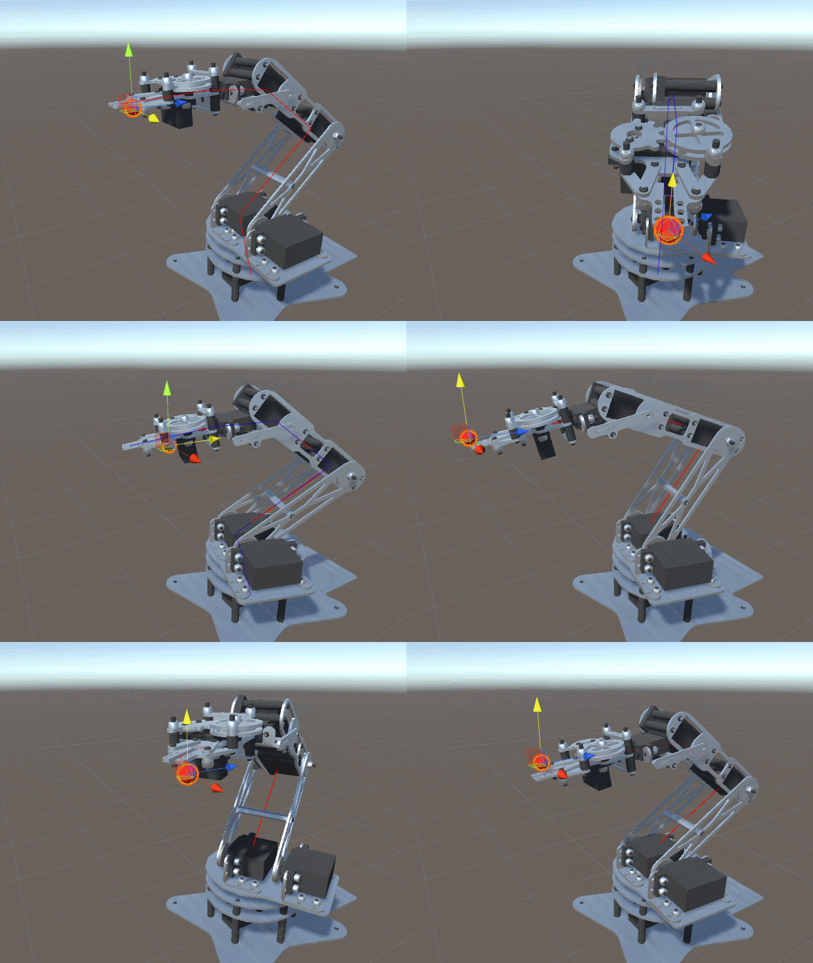
The other post in this series can be found here:DistanceFromTarget

Part 1. An Introduction to Procedural Animations
Part 2. The Mathematics of Forward Kinematics
Part 3. Implementing Forward Kinematics
Part 4. An Introduction to Gradient Descent
Part 5. Inverse Kinematics for Robotic Arms
Part 6. Inverse Kinematics for Tentacles
Part 7. Inverse Kinematics for Spider Legs 🚧 (work in progress!)

At the end of this post you can find a link to download all the assets and scenes necessary to replicate this tutorial.

Introduction

The previous post in this series, Implementing Forward Kinematics, provided a solution to the problem of Forward Kinematics. We have left with a function, called ForwardKinematics, which indicates which point in space our robotic arm is currently touching.

If we have a specific point in space that we want to reach, we can use ForwardKinematics to estimate how close we are, given the current joint configuration. The distance from the target is a function that can be implemented like this:

public float DistanceFromTarget(Vector3 target, float [] angles)
{
    Vector3 point = ForwardKinematics (angles);
    return Vector3.Distance(point, target);
}

Finding a solution for the problem of Inverse Kinematics means that we want to minimise the value returned from DistanceFromTarget. Minimising a function is one of most common problems, both in programming and Mathematics. The approach we will use relies on a technique called gradient descent (Wikipedia). Despite not being the most efficient, it has the advantage of being problem-agnostic and requires knowledge that most programmers already have.

❓ Solving Inverse Kinematics analytically

Gradient descent is an optimisation algorithms. It can be used for all those problems for which we do not have a proper equation. This is not our case, since we do have an equation for the forward kinematics, as derived in The Mathematics of Forward Kinematics:

$P_{i} = P_{i-1} + rotate\left(D_i, P_{i-1}, \sum_{k=0}^{i-1}\alpha_k\right)$

The distance from a target point $T$ is given by:

$D = \left | T - P_{effector}\right |$

where $\left | X\right |$ is the Euclidean norm of a vector $X$ .

An analytical solution to this problem can be found by minimising $D$ , which is a function of $\alpha$ .

There are other, more structured approaches to solve the problem of inverse kinematics. You can have a look at the Denavit-Hartenberg matrices (Wikipedia) to start.

Gradient Descent

The easiest way to understand how gradient descent works, is to imagine a hilly landscape. We find ourselves on a random location, and we want to reach its lowest point. We call that the minimum of the landscape. At each step, gradient descent tells you to move in the direction that lowers your altitude. If the geometry of the landscape is relatively simple, this approach will converge towards the bottom of the valley.

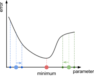
The diagram below shows a typical scenario in which gradient descent is successful. In this toy example, we have a function that takes a single parameter (X axis), and returns an error value (Y axis). Starting from random points on the X axis (blue and green points), gradient descent should force us to move in the direction of the minimum (blue and green arrows).

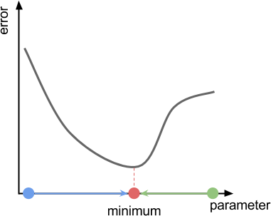
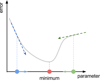
Looking at the function in its entirety, the direction in which we have to move is obvious. Unfortunately, gradient descent has no prior knowledge of where the minimum is. The best guess the algorithm can do is to move in the direction that of the slope, also called the gradient of the function. If you are on a hill, let a ball go and follow it to reach the valley. The diagram below shows the gradient of the error function at two different points.

❓ How does a good landscape look like?

In order for gradient descent to be effective, the function we are trying to minimise should satisfy certain properties. If the landscape of a function is relatively smooth, there is a higher chance for gradient descent to succeed. Functions that are discontinuous or have lot of peaks are particularly challenging, as we might have to take a longer journey to reach the bottom of the valley.

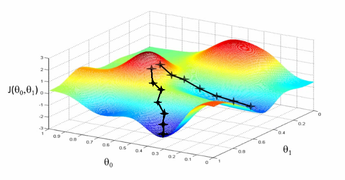
This is what the landscape for a robotic arm with two joints (controller by $\theta_0$ and $\theta_1$ might look like:

Gradient Estimation

If you have studied Calculus before, you might know the gradient of a function is deeply connected to its derivative. Calculating the derivative, however, requires the function to satisfy certain mathematical properties that, in general, cannot be guaranteed for arbitrary problems. Moreover, the analytical derivation of the derivative needs the error function to be presented analytically. Once again, you do not always have access to an analytical version of the function you are trying to minimise.

In all those cases, it is impossible to access the true derivative of the function. The solution is to give a rough estimate of its value. The diagram below shows how this can be done in one dimension. By sampling nearby points, you can get a feeling for the local gradient of the function. If the error function is smaller on the left, you go on the left. Likewise, if it is smaller on the right, you go on the right.

This sampling distance will be called $\Delta x$ in the following section.

❓ What’s the difference between the gradient and the derivative?

The concept of gradient and derivative are strictly related to each other.

The gradient or directional derivative of a function is a vector that points in the direction of the steepest ascent. In the case of one dimensional functions (like the ones shown in these diagrams) the gradient is either $+1$ or $-1$ if the function is going up or down, respectively. If a function is defined over two variables (for instance, a robotic arm with two joints) then the gradient is an “arrow” (a unit vector) of two elements which points towards the steepest ascent.

The derivative of a function, instead, is a single number that indicates how fast a function is rising when moving in the direction of its gradient.

In this tutorial, we do not aim to calculate the real gradient of the function. Instead, we provide an estimation. Out estimated gradient is a vector that, hopefully, indicates the direction or the steepest ascent. As we will see, it might not necessarily be of a unit vector.

❓ How critical is this sampling?

A lot. Sampling nearby points requires you to evaluate the function at a certain distance from your current position. This distance is critical.

Think about the following:

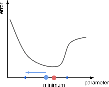
The sampling distance used to estimate the gradient is too large. Gradient descent incorrectly believes the right side is higher than the left one. The result is that the algorithm proceeds in the wrong direction.

Reducing the sampling distance attenuates this problem, but it never gets rid of it. Moreover, a smaller sampling distance causes a a slower convergence to a solution.

This problem can be solved by adopting more advanced versions of gradient descents.

❓ What if the function has several local minima?

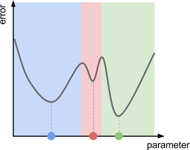
Generally speaking, such a greedy approach yields no guarantees that you will actually reach the bottom of a valley. If there are more valleys, you might get stuck in one of them, without being able to reach the actual target.

With the naive description of gradient descent that has been given so far, you could see this happening with the function in the diagram below. This function has three local minima, which represents three different valleys. If we initialise gradient descent using a point from the green region, we will end up at the bottom of the green valley. The same applies for the red and blue regions.

Once again, all of those problems are addressed by adopting more advanced versions of gradient descent.

The Maths

Now that we have a general understanding of how gradient descent works graphically, let’s see how this translates mathematically. The first step is to calculate the gradient of our error function $f$ at a specific point $p$ . What we need is to find the direction in which the function grows. The gradient of a function is deeply connected with its derivative. For this reason, a good starting point for our estimation is to investigate how the derivative is calculate in the first place.

Mathematically speaking, the derivative of $f$ is called ${f}'$ . It’s value at the point $p$ is ${f}'\left(p\right)$ , and it indicates how fast the function grows. It holds that:

${f}'\left(p\right) > 0 \Rightarrow f$ is going up, locally;
${f}'\left(p\right) < 0 \Rightarrow f$ is going down, locally;
${f}'\left(p\right) = 0 \Rightarrow f$ is flat, locally.

The idea is to use an estimation of ${f}'\left(p\right)$ to calculate the gradient, called $\nabla f$ . Mathematically, ${f}'$ is defined as:

${f}'\left(p\right) \right ) = \lim_{\Delta x \rightarrow 0} \frac{f\left(p+\Delta x\right) - f\left(p\right)}{\Delta x}$

The following diagram shows what this means:

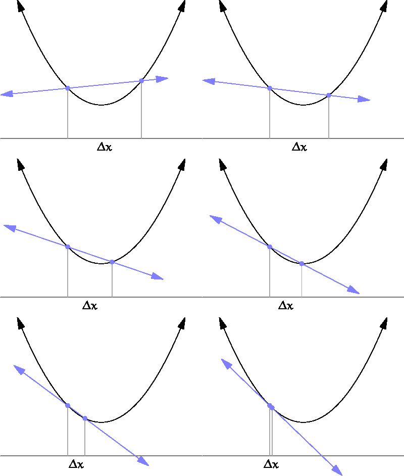For what we are concerned, to estimate the derivative we need to sample the error function at two different points. The small distance between them, $\Delta x$ is the sampling distance that we have introduced in the previous section.

To recap. The actual derivative of a function requires the usage of a limit. Our gradient is an estimation of the derivative, made using a sufficiently small sampling distance:

Derivative
${f}'\left(p\right) \right ) = \lim_{\Delta x \rightarrow 0} \frac{f\left(p+\Delta x\right) - f\left(p\right)}{\Delta x}$
Estimated gradient
$\nabla{f}\left(p\right) \right ) = \frac{f\left(p+\Delta x\right) - f\left(p\right)}{\Delta x}$

We will see in the next section how these two differ for functions with multiple variables.

Once we have found our estimated derivative, we need to move in its opposite direction to climb down the function. This means that we have to update our parameter $p$ like this:

$p_{i+1} = p_{i} - L \nabla {f}\left(p_i\right)$

The constant $L$ is often referred as learning rate, and it dictates how fast we move against the gradient. Larger values approach the solution faster, but are also more likely to overshoot it.

❓ lim?

If you have not studied Calculus, you might be unfamiliar with the notion of limits. Limits are mathematical tools that allows us to reach for infinity.

Think about our toy example. The smallest the sampling distance $\Delta_x$ is, the better we can estimate the actual gradient of the function. However, we can’t really set $\Delta_x=0$ , because divisions by zero are not allowed. Limits allow us to circumnavigate this issue. We cannot divide by zero, but with limits we can ask for a number that is arbitrarily close to zero, without ever being actually zero.

Multiple Variables

The solution we have found so far works on a single dimension. What it means is that we have given the definition of the derivative for a function of the type $f\left(p\right)$ , where $p$ is a single number. In this particular case, we could find a reasonably accurate estimate of the derivative by sampling the function $f$ at two points: $p$ and $p+\Delta x$ . The result is a single number that indicates if the function is increasing or decreasing. We have used this number as our gradient.

A function with a single parameter corresponds to robot arm with a single joint. If we want to perform gradient descent for more complex robotic arms, we need to define the gradient for functions on multiple variables. If our robotic arm has three joints, for instance, our function will look more like $f\left(\alpha_0, \alpha_1, \alpha_2\right)$ . In such a case, the gradient is a vector made out of three numbers, which indicate the local behaviour of $f$ in the 3D dimensional space of its parameters.

We can introduce the concept of partial derivatives, which essentially are “traditional” derivatives, calculated on a single variable at a time:

${f}'_{\alpha_0}\left(\alpha_0, \alpha_1, \alpha_2\right) \right )=\lim_{\Delta x \rightarrow 0} \frac{f\left(\alpha_0 + \Delta_x, \alpha_1, \alpha_2\right)-f\left(\alpha_0, \alpha_1, \alpha_2\right)}{\Delta x}$

${f}'_{\alpha_1}\left(\alpha_0, \alpha_1, \alpha_2\right) \right )=\lim_{\Delta y \rightarrow 0} \frac{f\left(\alpha_0, \alpha_1+\Delta_y, \alpha_2\right)-f\left(\alpha_0, \alpha_1, \alpha_2\right)}{\Delta y}$

${f}'_{\alpha_2}\left(\alpha_0, \alpha_1, \alpha_2\right) \right )=\lim_{\Delta z \rightarrow 0} \frac{f\left(\alpha_0, \alpha_1, \alpha_2+\Delta_z\right)-f\left(\alpha_0, \alpha_1, \alpha_2\right)}{\Delta z}$

They represent three different scalar numbers, each indicating how the function grows on a specific direction (or axes). To calculate our total gradient, we approximate each partial derivative with a correspondent gradient, using sufficiently small sampling distances $\Delta x$ , $\Delta y$ and $\Delta z$ :

$\nabla {f}_{\alpha_0}\left(\alpha_0, \alpha_1, \alpha_2\right) \right )=\frac{f\left(\alpha_0 + \Delta_x, \alpha_1, \alpha_2\right)-f\left(\alpha_0, \alpha_1, \alpha_2\right)}{\Delta x}$

$\nabla {f}_{\alpha_1}\left(\alpha_0, \alpha_1, \alpha_2\right) \right )=\frac{f\left(\alpha_0, \alpha_1+\Delta_y, \alpha_2\right)-f\left(\alpha_0, \alpha_1, \alpha_2\right)}{\Delta y}$

$\nabla {f}_{\alpha_2}\left(\alpha_0, \alpha_1, \alpha_2\right) \right )= \frac{f\left(\alpha_0, \alpha_1, \alpha_2+\Delta_z\right)-f\left(\alpha_0, \alpha_1, \alpha_2\right)}{\Delta z}$

For our gradient descent, we will use the vector that incorporates those three results as the gradient:

$\nabla f \left(\alpha_0, \alpha_1, \alpha_2\right) = \left[\nabla {f}_{\alpha_0}\left(\alpha_0, \alpha_1, \alpha_2\right),\nabla{f}_{\alpha_1}\left(\alpha_0, \alpha_1, \alpha_2\right) ,\nabla{f}_{\alpha_2}\left(\alpha_0, \alpha_1, \alpha_2\right)\right]$

❓ This is not a unit vector!

The directional derivative of a function is a unit vector that indicates the direction of its steepest ascent. Directions are vectors of unit length. However, it’s easy to see that the gradient that we have calculate here is not necessarily a unit vector.

While this might sounds like a mathematical abuse (and it probably is!) it is not necessarily a problem for our algorithm. What we need is a vector that points in the direction of the steepest ascent. Using an estimation of the partial derivatives as elements of such a vector satisfy our constraints. If we want this to be a unit vector, we can simply normalise it, by dividing it by its length.

Using a unit vector as the advantage that we know the maximum speed at which we move along the surface, which is the learning rate $L$ . Using a non normalised gradient means that we more faster or slower depending on the inclination of $f$ . This is neither good nor bad; it’s just a different approach to solve this problem.

📚 Recommended Books

Things to Make and Do in the Fourth Dimension

Humble Pi: A Comedy of Maths Errors

Love Triangle: The Life-changing Magic of Trigonometry

Other resources

The next part of this tutorial will finally show a working implementation of this algorithm.

Part 1. An Introduction to Procedural Animations
Part 2. The Mathematics of Forward Kinematics
Part 3. Implementing Forward Kinematics
Part 4. An Introduction to Gradient Descent
Part 5. Inverse Kinematics for Robotic Arms
Part 6. Inverse Kinematics for Tentacles
Part 7. Inverse Kinematics for Spider Legs 🚧 (work in progress!)

Become a Patron!
Patreon You can download the Unity project for this tutorial on Patreon.

Credits for the 3D model of the robotic arm goes to Petr P.

💖 Support this blog

This website exists thanks to the support of patrons on Patreon. If you think my work has helped or inspired you, please consider joining!

👉

Become a member

👈

Comments

10 responses to “An Introduction to Gradient Descent”

Bob

June 24, 2020

Hi, thank you for this explanation.
It is not really a big deal, but I think there are two missing “=” in the first formulas of the derivatives, before the limit.
Thanks again

Reply
1. Alan Zucconi
  
  July 3, 2020
  
  Thank you for spotting that, Bob!
  I have corrected the formulas!
  
  Reply
Dioinecail

December 19, 2017

There is a little mistake in the code?
As DistanceFromTarget returns float, not Vector3. Might confuse someone with very little experience in C#

Reply
1. Alan Zucconi
  
  December 20, 2017
  
  Thank you!
  
  Reply
Andrew C

August 29, 2017

Very interesting and useful, thanks. I think you need ∇fα₂ once in your final vector though, rather than ∇fα₀ twice.

Reply
1. Alan Zucconi
  
  August 30, 2017
  
  Thank you! 🙂
  
  Reply
Alan W

May 30, 2017

This is a lot to take in, had I not already completed higher level math courses at my university this would certainly be a much tougher read than it already is. You explained very thoroughly however, you must have a deep understanding of the topic. I appreciate the tutorial and am eager to learn more.

Reply
1. Alan Zucconi
  
  May 31, 2017
  
  Thank you!
  I wanted to give a more Maths-y introduction to the topic. Gradient Descent is often implemented in a very naive way. But it has solid theoretical foundations.
  
  Reply
An Introduction to Procedural Animations – Alan Zucconi

May 12, 2017

[…] Part 4. An Introduction to Gradient Descent […]

Reply
Implementing Forward Kinematics – Alan Zucconi

May 10, 2017

[…] of Forward Kinematics, we will see how to translate it into C# for Unity. The next tutorial, An Introduction to Gradient Descent, will finally show the theoretical foundations to solve inverse […]

Reply