Positioning and Trilateration

Follow @AlanZucconi

This post shows how it is possible to find the position of an object in space, using a technique called trilateration. The traditional approach to this problem relies on three measurements only. This tutorial addresses how to it is possible to take into account more measurements to improve the precision of the final result. This algorithm is robust and can work even with inaccurate measurements.

• Introduction
• Part 1. Geometrical Interpretation
• Part 2. Mathematical Interpretation
• Part 3. Optimisation Algorithm
• Part 4. Additional Considerations
• Conclusion

If you are unfamiliar with the concepts of latitude and longitude, I suggest you read the first post in this series: Understanding Geographical Coordinates.

Introduction

Finding the position in space of an object is hard. What makes such a simple request so complex, is the fact that no traditional sensor is able to locate an object. What most sensors do, usually, is estimating the distance from the target object. Sonars and radars send out sound waves and calculate the distance by detecting how long it takes for their signal to bounce back. Satellites basically do the the same, bur using radio waves. Estimating the distance from an object is often relatively easy to do.

The solution to locate an object is to rely on several distance measurements, taken by different sensors (or by the same sensor at different times). Sensor fusion is a very active field of research, and allows to reconstruct complex information from very simple measurement. The rest of this post will introduce the concept of trilateration, which is one of the most common techniques used to calculate the position of an object given distance measurements.

Geometrical Interpretation

Let’s imagine that we want to find the location of an object. Our first try relies on a beacon, or station, sitting at a known position . Both and are expressed with latitude and longitude values. The station cannot locate directly, but can estimate its relative distance .

With only one station available, we cannot identify the exact position of . What we know, however, is how close it is. Each point that is at distance from is a potential candidate for . This means that with only one beacon, our guess of is limited to a circle of radius around (below, in red).

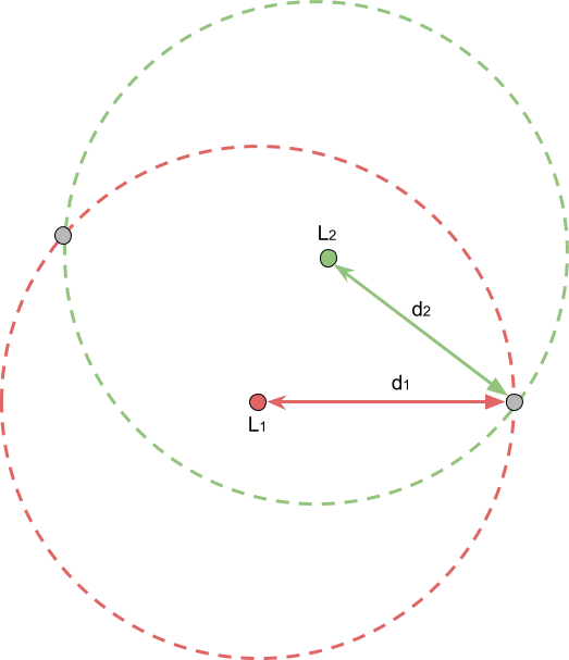
We can improve the situation by using not one but two beacons, and (below). Our object  can only be along the circumference of the red circle. But for the same reason, it can only be along the circumference of the green circle. This means that it has to be on the intersections of the two circles. This suddenly restricts our guess to only two possible locations (in grey).

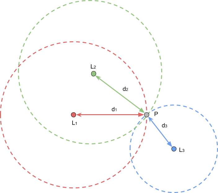
If we want to be absolutely precise, we need a third station, . The three circles will meet in only one point, which is indeed the correct location of .

In order to do that, we have a set of  beacons or stations, each one at a known locations . Each beacon can sense its distance from , which is called .

Mathematical Interpretation

A point on the Cartesian plane lies on a circle of radius centred at if and only if is a solution to this equation:

With the same reasoning, we can derive equations for the circles generated by the beacons. Each one has its own position, expressed with latitude and longitudes coordinates, , and , respectively.

The problem of trilateration is solved mathematically by finding the point that simultaneously satisfies the equations of these three circles.

There are several ways to solve these equations. If you are interested in the actual derivation, Wikipedia has a nice page explaining each step.

Optimisation Algorithm

While it is definitely true that trilateration can be seen (and solved) as a geometrical problem, this is often impractical. Relying on the mathematical modelling seen in the previous section requires us to have an incredibly high accuracy on our measurements. Worst case scenario: if the circles do not meet in a single point, the set of equations will have no solution. This leaves us with nothing. Even assuming we do have perfect precision, the mathematical approach does not scale nicely. What is we have not three, but four points? What if we have one hundred?

The problem of trilateration can be approached from an optimisation point of view. Ignoring circles and intersections, which is the point that provides us with the best approximation to the actual position ?

Given a point , we can estimate how well it replaces . We can do this simply by calculating its distance from each beacon . If those distances perfectly match with their respective distances , then is indeed . The more deviates from these distances, the further it is assumed from .

Under this new formulation, we can see trilateration as an optimisation problem. We need to find the pint that minimise a certain error function. For our , we have not one by three sources of error: one for each beacon:

A very common way to merge these different contributions is to average their squares. This takes away the for possibility of negative and positive errors to cancel each others out, as squares are always positive. The quantity obtained is known as mean squared error:

What is really nice about this solution is that it can be used to take into account an arbitrary number of points. The piece of code below calculates the mean square error of a point x, given a list of locations and their relative distances from the actual target.

# Mean Square Error
# locations: [ (lat1, long1), ... ]
# distances: [ distance1, ... ]
def mse(x, locations, distances):
	mse = 0.0
	for location, distance in zip(locations, distances):
		distance_calculated = great_circle_distance(x[0], x[1], location[0], location[1])
		mse += math.pow(distance_calculated - distance, 2.0)
	return mse / len(distances)

What’s left now is to find the point x that minimises the mean square error. Luckily, scipy comes with several optimisation algorithms that we can use.

# initial_location: (lat, long)
# locations: [ (lat1, long1), ... ]
# distances: [ distance1,     ... ] 
result = minimize(
	mse,                         # The error function
	initial_location,            # The initial guess
	args=(locations, distances), # Additional parameters for mse
	method='L-BFGS-B',           # The optimisation algorithm
	options={
		'ftol':1e-5,         # Tolerance
		'maxiter': 1e+7      # Maximum iterations
	})
location = result.x

Additional Considerations

While optimisations algorithms can solve many problems, it is unrealistic to expect them to perform well if we provide little to no additional information to them. One of the most important aspect is the initial guess. For a problem this straightforward, any relatively good optimisation algorithm should converge to a reasonable solution. However, providing a good starting point could reduce its execution time significantly.

There are several initial guesses that one could use. A sensible one is to use the centre of sensor which detected the closest distance.

	# Initial point: the point with the closest distance
	min_distance     = float('inf')
	closest_location = None
	for member in data:
		# A new closest point!
		if member['distance'] < min_distance:
			min_distance = member['distance']
			closest_location = member['location']
	initial_location = closest_location

Alternatively, one could average the locations of the sensors. If they are arranged in a grid fashion, this could work well. In the end, you should test which strategy works best for you.

Conclusion

This post concludes the series on localisation and trilateration.

• Part 1. Understanding Geographical Coordinates
• Part 2. Positioning and Trilateration

💖 Support this blog

This website exists thanks to the contribution of patrons on Patreon. If you think these posts have either helped or inspired you, please consider supporting this blog.

Follow @AlanZucconi

📧 Stay updated

You will be notified when a new tutorial is released!

Email:

Leave this field empty if you're human:

📝 Licensing

You are free to use, adapt and build upon this tutorial for your own projects (even commercially) as long as you credit me.

You are not allowed to redistribute the content of this tutorial on other platforms, especially the parts that are only available on Patreon.

If the knowledge you have gained had a significant impact on your project, a mention in the credit would be very appreciated. ❤️🧔🏻