Improving the Rainbow – Part 2

Follow @AlanZucconi

In the previous part of this tutorial, Improving the Rainbow – Part 1, we have seen different techniques to reproduce the colours of the rainbow procedurally. Solving this problem efficiently will allow us to simulate physically based reflections with a much higher fidelity.

The purpose of this post is to introduce a novel approach that yields better results than any of the previous solutions, without using any branching.

You can find the complete series here:

• Part 1. The Nature of Light
• Part 2. Improving the Rainbow (Part 1)
• Part 3. Improving the Rainbow (Part 2)
• Part 4. Understanding Diffraction Grating
• Part 5. The Mathematics of Diffraction Grating
• Part 6. CD-ROM Shader: Diffraction Grating (Part 1)
• Part 7. CD-ROM Shader: Diffraction Grating (Part 2)
• Part 8. Iridescence on Mobile
• Part 9. The Mathematics of Thin-Film Interference
• Part 10. Car Paint Shader: Thin-Film Interference

A link to download the Unity project used in this series is also provided at the end of the page.

Introduction

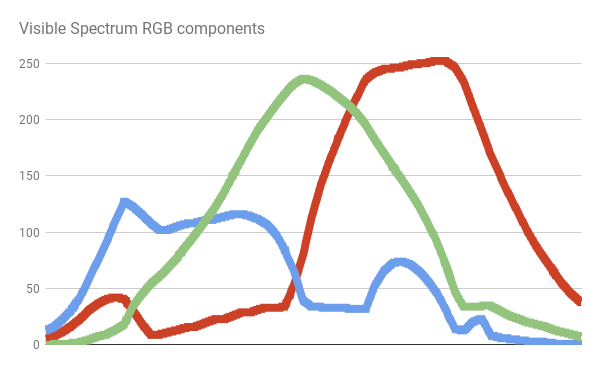
In the previous post, we have analysed four different techniques to convert wavelengths in the visible range of the electromagnetic spectrum (400-700 nanometers) to their respective colours.

Three of those solutions (JET, Bruton and Spektre) heavily relied on if statements. While that is a standard practice in C#, branching in a shader is notoriously bad. The approach discussed in the GPU Gems book is the only one that did not use any branching. Despite that, it did not provide the best approximation for the colours in the visible spectrum.

Name	Gradient
GPU Gems
Visible

The post will show an optimised version of the colour scheme firstly described in the GPU Gems book.

The “Bump” Colour Scheme

The original colour scheme introduced in the GPU Gems book used three parabolas (called “bumps” by the author) to replicate the distribution of R, G and B colours in the rainbow.

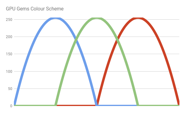
Each bump is described by the following equation:

Each wavelength in the range [400, 700] is associated with a normalised value in the range [0,1]. Then, the R, G and B components of the visible spectrum are given by:

All the numerical values have been been chosen by the author experimentally. You can see, however, how poorly they map to the actual distribution of colours.

Optimising for Quality

The first solution I personally came up with uses exactly the same equations of the GPU Gems colour scheme. However, I have optimised all the numerical values so that the final range of colours matches as closely as possible with the actual colours from the visible spectrum.

The result converges to the following solution:

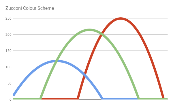
And yields a much more realistic result:

Name	Gradient
GPU Gems
Zucconi
Visible

Like the original solution, this new approach is branchless. Hence, it is perfect for shaders. This is the code:

// Based on GPU Gems
// Optimised by Alan Zucconi
inline fixed3 bump3y (fixed3 x, fixed3 yoffset)
{
	float3 y = 1 - x * x;
	y = saturate(y-yoffset);
	return y;
}
fixed3 spectral_zucconi (float w)
{
    // w: [400, 700]
	// x: [0,   1]
	fixed x = saturate((w - 400.0)/ 300.0);

	const float3 cs = float3(3.54541723, 2.86670055, 2.29421995);
	const float3 xs = float3(0.69548916, 0.49416934, 0.28269708);
	const float3 ys = float3(0.02320775, 0.15936245, 0.53520021);

	return bump3y (	cs * (x - xs), ys);
}

Improving the Rainbow

If we look closer at the distribution of colours in the visible spectrum, we can notice that parabolas cannot really capture the R, G and B colour curves. A slightly better approach is to use six parabolas, instead of just three. Fitting two bumps for each primary component, we can get a much better approximation. The difference is really visible in the violet part of the spectrum.

The difference is really visible in the violet and orange parts of the spectrum:

Name	Gradient
Zucconi
Zucconi6
Visible

Here is the code:

// Based on GPU Gems
// Optimised by Alan Zucconi
fixed3 spectral_zucconi6 (float w)
{
	// w: [400, 700]
	// x: [0,   1]
	fixed x = saturate((w - 400.0)/ 300.0);

	const float3 c1 = float3(3.54585104, 2.93225262, 2.41593945);
	const float3 x1 = float3(0.69549072, 0.49228336, 0.27699880);
	const float3 y1 = float3(0.02312639, 0.15225084, 0.52607955);

	const float3 c2 = float3(3.90307140, 3.21182957, 3.96587128);
	const float3 x2 = float3(0.11748627, 0.86755042, 0.66077860);
	const float3 y2 = float3(0.84897130, 0.88445281, 0.73949448);

	return
		bump3y(c1 * (x - x1), y1) +
		bump3y(c2 * (x - x2), y2) ;
}

There is no doubt that spectral_zucconi6 provides the best colour approximation, without introducing any branching. If performance is an issue, you can rely upon its simplified version spectral_zucconi.

Conclusion

This post provides an overview of some of the most common techniques to generate rainbow-like patterns in a shader. Moreover, a novel approach has been introduced.

Name	Gradient
JET
Bruton
GPU Gems
Spektre
Zucconi
Zucconi6
Visible

You can find a WebGL port of those colour schemes on this Shadertoy page.

You can find the complete series here:

• Part 1. The Nature of Light
• Part 2. Improving the Rainbow (Part 1)
• Part 3. Improving the Rainbow (Part 2)
• Part 4. Understanding Diffraction Grating
• Part 5. The Mathematics of Diffraction Grating
• Part 6. CD-ROM Shader: Diffraction Grating (Part 1)
• Part 7. CD-ROM Shader: Diffraction Grating (Part 2)
• Part 8. Iridescence on Mobile
• Part 9. The Mathematics of Thin-Film Interference
• Part 10. Car Paint Shader: Thin-Film Interference

Become a Patron!
You can download the Unity package for the CD-ROM Shader effect on Patreon.
The Python project used to find the optimal parameters for the spectral_zucconi and spectral_zucconi6 functions is available on Patreon as well.

💖 Support this blog

This website exists thanks to the contribution of patrons on Patreon. If you think these posts have either helped or inspired you, please consider supporting this blog.

Follow @AlanZucconi

📧 Stay updated

You will be notified when a new tutorial is released!

Email:

Leave this field empty if you're human:

📝 Licensing

You are free to use, adapt and build upon this tutorial for your own projects (even commercially) as long as you credit me.

You are not allowed to redistribute the content of this tutorial on other platforms, especially the parts that are only available on Patreon.

If the knowledge you have gained had a significant impact on your project, a mention in the credit would be very appreciated. ❤️🧔🏻