The Mathematics of Rayleigh Scattering

This post introduces the Mathematics of Rayleigh Scattering, which is the optical phenomenon that causes the sky to appear blue. The equations derived in this tutorial will be translated into shader code in the next tutorial.

You can find all the post in this series here:

Part 1. Volumetric Atmospheric Scattering
Part 2. The Theory Behind Atmospheric Scattering
Part 3. The Mathematics of Rayleigh Scattering
Part 4. A Journey Through the Atmosphere
Part 5. A Shader for the Atmospheric Sphere
Part 6. Intersecting The Atmosphere
Part 7. Atmospheric Scattering Shader
🔒 Part 8. An Introduction to Mie Theory

You can download the Unity package for this tutorial at the bottom of the page.

Introduction

In the previous tutorial, we have derived an equation that provides a good framework to approximate atmospheric scattering in a shader. What we have omitted, however, is the fact that a single equation will not yield believable results. If we want an atmospheric shader that looks good, we have to step up our Maths.

The interaction between light and matter is extremely complex, and there is no easy way to fully describe it. Modelling atmospheric scattering is, in fact, exceptionally difficult. Part of the problem comes from the fact that the atmosphere is not a homogeneous medium. Both its density and composition change significantly as a function of the altitude, making it virtually impossible to come up with a “perfect” model.

This is why the scientific literature presents several models of scattering, each one designed to describe a subset of optical phenomena occurring under specific conditions. Most optical effects that planets exhibit can be reproduced by taking into consideration two different models: Rayleigh scattering and Mie scattering. Those two mathematical tools allow predicting how light scatters on objects of different size. The former models how light is reflected by the oxygen and nitrogen molecules that make up most of the air. The latter, models how light reflects on much larger compounds that are suspended in the lower atmosphere, such as pollen, dust and pollutants.

Rayleigh scattering causes the sky to be blue, and sunsets to be red. Mie scattering gives clouds their white colour. If you want to understand how, we’ll have to delve deeper into the mathematics of scattering.

Rayleigh Scattering

What is the fate of a photon that hits a particle? To answer this question, we first need to redefine it in a more formal way. Let’s imagine a ray of light travelling through empty space, suddenly colliding with a particle. The outcome of such a collision varies dramatically depending on the size of the particle and the colour of the light. If the particle is small enough (such as atoms and molecules) the behaviour of the light is best predicted by the Rayleigh scattering.

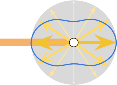
What happens is that a part of the light continues its journey unaffected. However, a small percentage of that original light interact with the particle and get scattered in all directions. Not all directions, however, receive an equal amount of light. Photons are more likely to pass straight through the particle or to bounce back. Conversely, the less likely outcome for a photon is being deflected by 90 degrees. Such a behaviour can be seen in the diagram below. The blue line shows the preferred directions for the scattered light.

This optical phenomenon is described mathematically by the Rayleigh scattering equation $S \left(\lambda, \theta, h \right )$ , which tells the ratio of the original light $I_0$ that is scattered towards the direction $\theta$ :

$I = I_0 \, S \left(\lambda, \theta, h\right)$

$S \left(\lambda, \theta, h\right ) = \frac{\pi^2 \left(n^2-1 \right )^2}{2} \underset{\text{density}}{\underbrace{\frac{\rho\left(h\right)}{N}}} \overset{\text{wavelength}}{\overbrace{\frac{1}{\lambda^4}}} \underset{\text{geometry}}{\underbrace{\left(1+\cos^2\theta \right )}}$

Where:

$\lambda$ : the wavelength of the incoming light;
$\theta$ : the scattering angle;
$h$ : the altitude of the point;
$n=1.00029$ : the refractive index of air;
$N=2.504 \cdot 10^{25}$ : the molecular number density of the standard atmosphere. This is the number of molecules per cubic metre;
$\rho\left(h\right)$ : the density ratio. This number is equal to $1$ at sea level, and decreases exponentially with $h$ . There is a lot to say about this function, and we will do it in a future post of this series.

❓ That is not the equation for the Rayleigh scattering!

If you have encountered the Rayleigh scattering in a field other than computer graphics, chances are that you have seen a different equation. The one that Wikipedia presents on its Rayleigh scattering entry, for instance, looks rather different.

The equation used in this tutorial comes from the scientific paper Display of The Earth Taking into Account Atmospheric Scattering, by Nishita et al..

❓ Where does this function come from?

One of the missions of this blog is to provide a derivation of all the quantities introduced. Unfortunately, this will not be the case for the equations that govern the Rayleigh scattering.

If you are still curious to understand why light particles reflect in such a bizarre way onto air molecules, the following explanation might give you an intuition into what’s really going on.

Rayleigh scattering is not really caused by light “bouncing off” particles. Light is an electromagnetic wave, and it can interact with the charge imbalances that are naturally present in certain molecules. Those charges become excited by the absorption of the incoming electromagnetic radiation, which is later re-emitted. The two-lobed shape you see in the phase function shows that air molecules become electric dipoles, radiating like exactly like microscopic antennas.

The first thing we have noticed about the Rayleigh scattering is that certain directions receive more light than others. The second important aspect is that the amount of light scattered is strongly dependent on the wavelength $\lambda$ of the incoming light. The polar diagram below visualises $S \left(\lambda, \theta\right, 0 )$ for three different wavelengths. Evaluating $S$ with $h=0$ is often referred to as scattering at sea level.

The image below shows a rendering of the scattering coefficients for a continuous range of wavelength/colour of the visible spectrum (code available on ShaderToy).

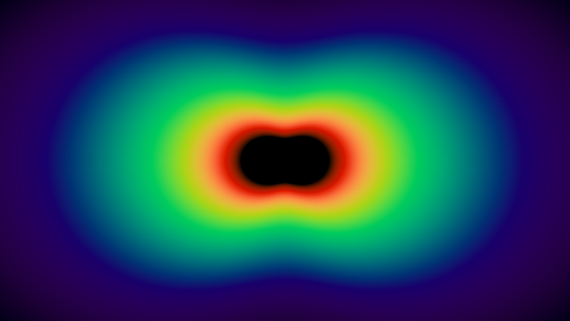
The centre of the image appears is black because wavelengths in that range are outside the visible spectrum.

Rayleigh Scattering Coefficient

The equation for the Rayleigh scattering indicates how much light is scattered towards a particular direction. It does not tell, however, how much energy is scattered in total. To calculate that, we need to take into account the energy dispersion in all directions. Such a derivation is not for the faint-hearted; if you are not comfortable with advanced Calculus, this is the result:

$\beta \left(\lambda, h \right )=\frac{8\pi^3 \left(n^2-1 \right )^2}{3} \frac{\rho\left(h\right)}{N} \frac{1}{\lambda^4}$

Where $\beta \left(\lambda, h \right )$ indicates the fraction of the energy that is lost to scattering after a collision with a single particle. This is often referred as the Rayleigh scattering coefficient.

If you have read the previous part of this tutorial, you might have guessed that $\beta$ is indeed the extinction coefficient used in the definition of the transmittance $T\left(\overline{AB}\right)$ over a segment $\overline{AB}$ .

Unfortunately, calculating $\beta$ is very expensive. In the shader that we are going to write, we will try to save as much computation as possible. For this reason, it is useful to “extract” from the scattering coefficient all the factors that are constant. This leaves us with $\beta \left(\lambda\right )$ , which is known as the Rayleigh scattering coefficient as sea level ( $h=0$ ):

$\beta \left(\lambda \right )=\frac{8\pi^3 \left(n^2-1 \right )^2}{3} \frac{1}{N} \frac{1}{\lambda^4}$

❓ Show me the Maths!

The equation for the Rayleigh scattering indicates the ratio of energy that is lost in a specific direction. To calculate the total loss, we need to take into account all the possible directions. A summation over a continuous interval requires an integration.

One might try to integrate $S \left(\lambda, \theta, h\right )$ over $\theta$ in the interval $\left[0,2\pi\right]$ , but that would be a mistake.

Despite the fact that we have been visualising the Rayleigh scattering in two dimensions, it actually is a three-dimensional phenomenon. The scattering angle $\theta$ can be any direction in a 3D space. Accounting for the total contribution of a function that depends on an angle $\theta$ in a 3D space (like $S$ ) is referred to as solid angle integration:

$\beta \left(\lambda, h \right ) = \int_{0}^{2\pi} \int_{0}^{\pi} S \left(\lambda, \theta, h \right ) \sin\theta \, d\theta d\phi$

The inner integral moves $\theta$ in the XY plane, while the outer integral rotates the result around the X axis to account for the third dimension. The added $\sin \theta$ is used for spherical angles.

The integration processs is only interested in what depends on $\theta$ . Several terms in $S \left(\lambda, \theta, h \right )$ are constant, and can be moved out of the integral:

$\beta \left(\lambda, h \right )=\int_{0}^{2\pi} \int_{0}^{\pi} \underset{\text{constant}}{\underbrace{ \frac{\pi^2 \left(n^2-1 \right )^2}{2} \frac{\rho\left(h\right)}{N} \frac{1}{\lambda^4} }} \left(1+\cos^2\theta \right ) \sin\theta \, d\theta d\phi=$

$=\frac{\pi^2 \left(n^2-1 \right )^2}{2} \frac{\rho\left(h\right)}{N} \frac{1}{\lambda^4} \int_{0}^{2\pi} \int_{0}^{\pi} \left(1+\cos^2\theta \right ) \sin\theta \, d\theta d\phi$

This massively simplifies the inner integral, which can now be performed:

$\beta \left(\lambda, h \right )=\frac{\pi^2 \left(n^2-1 \right )^2}{2} \frac{\rho\left(h\right)}{N} \frac{1}{\lambda^4} \int_{0}^{2\pi} \boxed{ \int_{0}^{\pi} \left(1+\cos^2\theta \right ) \sin\theta \, d\theta }d\phi=$

$=\frac{\pi^2 \left(n^2-1 \right )^2}{2} \frac{\rho\left(h\right)}{N} \frac{1}{\lambda^4} \int_{0}^{2\pi} \boxed{\frac{8}{3}} d\phi$

We can now perfom the outer integration:

$\beta \left(\lambda, h \right )=\frac{\pi^2 \left(n^2-1 \right )^2}{2} \frac{\rho\left(h\right)}{N} \frac{1}{\lambda^4} \boxed{ \int_{0}^{2\pi} \frac{8}{3} d\phi}=$

$=\frac{\pi^2 \left(n^2-1 \right )^2}{2} \frac{\rho\left(h\right)}{N} \frac{1}{\lambda^4} \boxed{ \frac{16 \pi}{3}}$

Which leads to the final form:

$\beta \left(\lambda, h \right )=\frac{8\pi^3 \left(n^2-1 \right )^2}{3} \frac{\rho\left(h\right)}{N} \frac{1}{\lambda^4}$

Since this is an integral that takes into account the scattering contributions in every direction, it makes sense that the expression does not depend on $\theta$ anymore.

This new equation provides yet another way to understand how different colours of light get scattered. The chart below shows the amount of scattering light is subjected to, as a function of its wavelength.

It is the strong relationship between the scattering coefficient $\beta$ and $\lambda$ which, ultimately, turns sunset skies red. The photons that we receive from the sun are distributed across a wide range of wavelengths. What the Rayleigh scattering tells us, is that atoms and molecules from Earth’s atmosphere scatter blue light more strongly than green or red. If light is allowed to travel long for long enough, all of its blue light will be lost by scattering. This is exactly what happens at sunset, when light is travelling almost parallel to the surface.

With the same reasoning, we can understand why the sky appears blue. The light from the sun arrives with a specific direction. However, its blue component is scattered in every direction. When you are looking at the sky, blue light is coming from every direction.

Rayleigh Phase Function

The original equation that describes the Rayleigh scattering, $S \left(\lambda, \theta\right )$ can be decomposed into two components. One is the scattering coefficient that we have just derived, $\beta \left(\lambda\right )$ , which modules its intensity. The second part is related to the geometry of the scattering, and controls its direction:

$S \left(\lambda, \theta, h\right ) = \beta \left(\lambda, h\right ) \gamma \left(\theta\right)$

This new quantity $\gamma \left(\theta\right)$ can be obtained dividing $S \left(\lambda, \theta, h\right )$ by $\beta \left(\lambda\right )$ :

$\gamma \left(\theta\right) = \frac{S \left(\lambda, \theta, h\right )} {\beta \left(\lambda\right )}=$

$= \underset{S \left(\lambda, \theta, h\right )}{\underbrace{ \frac{\pi^2 \left(n^2-1 \right )^2}{2} \frac{\rho\left(h\right)}{N} \frac{1}{\lambda^4} \left(1+\cos^2\theta \right ) }} \, \underset{\frac{1}{\beta \left(\lambda\right )}}{\underbrace{ \frac{3}{8\pi^3 \left(n^2-1 \right )^2} \frac{N}{\rho\left(h\right)} \lambda^4 }}=$

$= \frac{3}{16\pi} \left(1+\cos^2 \theta\right)$

You can see that this new expression does not depend on the wavelength of the incoming light. This might seem counter-intuitive, since we definitely know that the Rayleigh scattering affects shorter wavelenghts more.

What $\gamma \left(\theta\right)$ models, however, is the shape of the dipole that we have seen before. The term $\frac{3}{16\pi}$ serves as a normalisation factor, so that the integral over all possible angles $\theta$ sums up to $1$ . More technically, one can say that the integral over $4\pi$ steradians is $1$ .

We will see in the upcoming parts how separating these two components will allow deriving more efficient equations.

A Quick Recap

Rayleigh scattering equation: indicates the ratio of light that is deflected in the direction $\theta$ . The intensity of the scattering depends on the wavelength $\lambda$ of the incoming light.

$S \left(\lambda, \theta, h\right ) = \frac{\pi^2 \left(n^2-1 \right )^2}{2} \frac{\rho\left(h\right)}{N} \frac{1}{\lambda^4} \left(1+\cos^2\theta \right )$

Also:

$S \left(\lambda, \theta, h\right ) = \beta \left(\lambda,h \right ) \gamma\left(\theta\right)$

Rayleigh scattering coefficient: it indicates the ratio of light that is lost to scattering after a single collision.

$\beta \left(\lambda,h \right )=\frac{8\pi^3 \left(n^2-1 \right )^2}{3} \frac{\rho\left(h\right)}{N} \frac{1}{\lambda^4}$

Rayleigh scattering coefficient at sea level: it is equivalent to $\beta \left(\lambda,0\right )$ . Creating this additional coefficient will be very helpful to derive more efficient equations.

$\beta \left(\lambda \right )=\beta \left(\lambda,0 \right )=\frac{8\pi^3 \left(n^2-1 \right )^2}{3} \frac{1}{N} \frac{1}{\lambda^4}$

If we consider the wavelengths which loosely maps to red, green and blue colours, we obtain the following results:

$\beta\left(680nm\right) = 0.00000519673$

$\beta\left(550nm\right) = 0.0000121427$

$\beta\left(440nm\right) = 0.0000296453$

These results are calculate assuming $h=0$ (which implies $\rho=1$ ). This only happens at sea level, where the scattering coefficient is at its maximum value. Hence, it serves as a “baseline” for how much light is scattered.

Rayleigh phase function: controls the scattering geometry, which indicates the relative ratio of light lost in a particular direction. The $\frac{3}{16\pi}$ coefficient serves as a normalisation factor, so that the integral over a unit sphere is $1$ .

$\gamma\left(\theta\right)= \frac{3}{16\pi} \left(1+\cos^2 \theta\right)$

Density ratio: this is a function that is used to model the density of the atmosphere. It will be formally introduced in a future post. If you do not mind Maths spoilers, it is defined as:

$\rho\left(h\right)=exp\left\{-\frac{h}{H}\right\}$

where $H=8500$ metres is called the scale height.

Coming Next…

This tutorial introduced the concept and the Mathematics of Rayleigh Scattering. In the next one, we will explain how to model Earth’s atmosphere in an effective way. For now, we will only focus on the Rayleigh scattering. The last post in this series, An Introduction to Mie Theory, will complete the shader by adding a second type of scattering.

You can find all the post in this series here:

Part 1. Volumetric Atmospheric Scattering
Part 2. The Theory Behind Atmospheric Scattering
Part 3. The Mathematics of Rayleigh Scattering
Part 4. A Journey Through the Atmosphere
Part 5. A Shader for the Atmospheric Sphere
Part 6. Intersecting The Atmosphere
Part 7. Atmospheric Scattering Shader
🔒 Part 8. An Introduction to Mie Theory

A big thanks goes to Stephen Lavelle, who kindly helped with the derivations.

Download

Become a Patron!
You can download all the assets necessary to reproduce the volumetric atmospheric scattering presented in this tutorial.

Feature	Standard	Premium
Volumetric Shader	✅	✅
Clouds Support	❌	✅
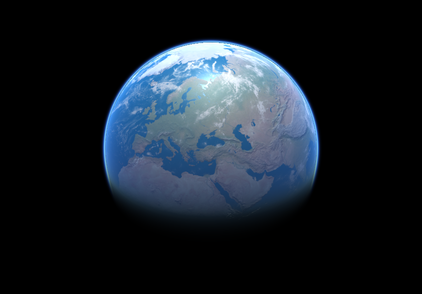
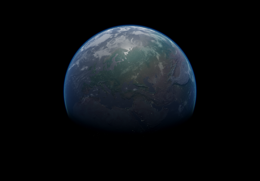
Day & Night Cycle	❌	✅
Earth 8K	✅	✅
Mars 8K	❌	✅
Venus 8K	❌	✅
Neptune 2K	❌	✅
Postprocessing	❌	✅
Download	Standard	Premium

💖 Support this blog

This website exists thanks to the contribution of patrons on Patreon. If you think these posts have either helped or inspired you, please consider supporting this blog.

Follow @AlanZucconi

📧 Stay updated

You will be notified when a new tutorial is released!

📝 Licensing

You are free to use, adapt and build upon this tutorial for your own projects (even commercially) as long as you credit me.

You are not allowed to redistribute the content of this tutorial on other platforms, especially the parts that are only available on Patreon.

If the knowledge you have gained had a significant impact on your project, a mention in the credit would be very appreciated. ❤️🧔🏻

Marco

July 22, 2018

Apologies for the bother but looks like the cheatsheet goes 404.

Reply to Marco
- Alan Zucconi
  
  July 22, 2018
  
  Hi Marco!
  Thank you, unfortunately I haven’t had time to complete that yet!
  
  Reply to Alan
Alexander

April 3, 2019

Hi Alan! Thank you for the great tutorial! I don’t quite understand how the density ratio and the molecular number density of the standard atmosphere work together in the represented Rayleigh scattering equation S(lambda, theta, h). The density of the atmosphere decreases exponentially with h starting from a certain value at the sea level. This relation can be written as p(h) = N*exp(-h/Ho), where N and Ho can be chosen arbitrary from the range {N >= 0, Ho > 0}. So, to visualize some kind of weak atmosphere I can set N to a smaller value than the density of the standard atmosphere. The smaller the value of N, the less the overall scattering effect of the atmosphere. But in the represented equation this relation is inverted and overall scattering effect of the atmosphere increases with decreasing N, which looks rather strange to me.

Reply to Alexander

Webmentions

Sprite Doodle Shader Effect - Alan Zucconi April 3, 2019

[…] my blog, I tend to cover rather advanced topics, from the mathematics of inverse kinematics to atmospheric Rayleigh scattering. Making such complex subjects understandable to a larger audience is something that I find very […]

Published

October 10, 2017

Alan Zucconi in Maths, Science, Tutorial | October 10, 2017