
This tutorial starts our journey into the world of inverse kinematics. There are countless ways to approach this problem, but they all starts with forward kinematics.
Inverse kinematics takes a point in space, and tells you how to move your arm to reach it. Forward kinematics solves the opposite, dual problem. Knowing how you are moving your arm, it tells which point in space it reaches.
The other post in this series can be found here:
- Part 1. An Introduction to Procedural Animations
- Part 2. The Mathematics of Forward Kinematics
- Part 3. Implementing Forward Kinematics
- Part 4. An Introduction to Gradient Descent
- Part 5. Inverse Kinematics for Robotic Arms
- Part 6. Inverse Kinematics for Tentacles
- Part 7. Inverse Kinematics for Spider Legs 🚧 (work in progress!)
At the end of this post you can find a link to download all the assets and scenes necessary to replicate this tutorial.
Robotic Arm
Inverse kinematics has been originally applied to control robotic arms. For this reason, this tutorial will make assumptions and use terminology related to robotics. This, however, does not limit the possible applications of inverse kinematics. Non-robotic scenarios, such as human arms, spider spiders and tentacles, are still possible.
First of all, let’s start showing what we mean with the term “robotic arm”:
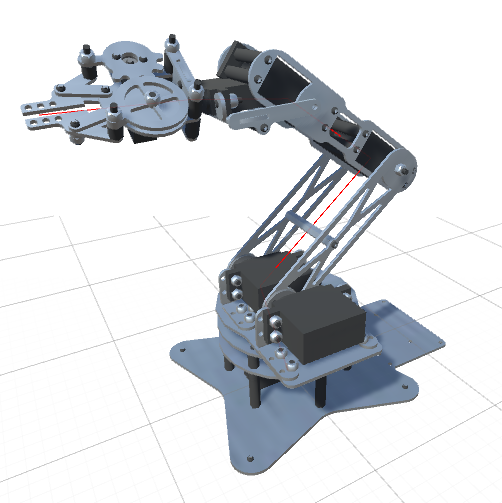
The picture above shows a typical robotic arm, made of “limbs” connected by “joints”. Since the robotic arm from the picture has five independent joints, it is said to have five degrees of freedom. Each joint is controller by a motor, which allows to moves the connected link to a certain angle.
Without losing generalisation, we can draw a precise schematics of the joints. In this particular tutorial, we will assume that each joint can only rotate on a single axis.
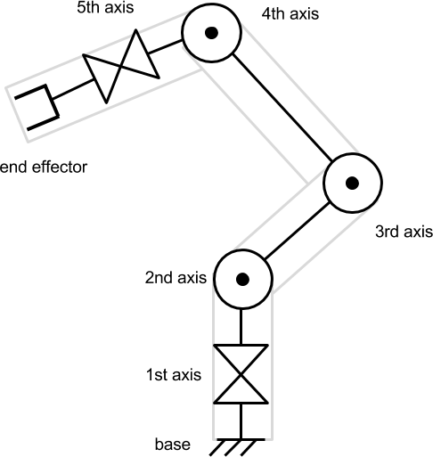
The tool attached at the end of the robotic arm is known as end effector. Depending on the context, it can be counted or not as a degree of freedom. In this tutorial, the end effector will not be considered since we will focus solely on the reaching movement.
Forward Kinematics
In this toy example, each joint is able to rotate on a specific axis. The state of each joint is hence measured as an angle. By rotating each joint to a specific angle, we cause the end effector to reach different points in space. Knowing where the end effector is, given the angles of the joints, is known as forward kinematics.
The forward kinematics is an “easy” problem. This means that for each set of angles, there is one and only one result, which can be calculated with no ambiguity. Understanding how a robotic arm moves depending on the inputs we provide to its motors is an essential step to find a solution to its dual problem of inverse kinematics.
Geometrical Interpretation
Before writing even a single line of code, we need to understand the Mathematics behind forward kinematics. And even before that, we need to understand what that means spatially and geometrically.
Since visualising rotations in 3D is not that easy, let’s start with a simple robotic arm that lies in a 2D space. A robotic arm has a “resting position”; that is the configuration when all the joints are rotated back to their “zero angle”.

The diagram above shows a robotic arm with three degrees of freedom. Each joint is rotated to its zero angle, resulting in this initial configuration. We can see how such configuration changes by rotating the first joint at  by
by  degrees. This causes the entire chain of joints and links anchored to to move accordingly.
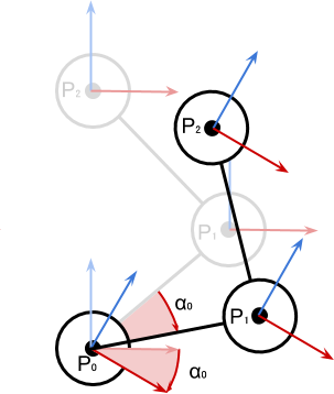
It is important to notice that the motors attached to other joints have not moved. Each joint contributes to the local rotation of its forward chain of links. The following diagram shows how the configuration changes when the second joint rotates by  degrees.
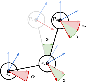
While only determines the position of  ,
,  is affected by both and . The rotational frame of reference (the red and blue arrows) are oriented according to the sum of the rotations of the earlier chain of links they are connected to.
The Maths
From the previous diagrams it should be clear to solve the problem of forward kinematics, we need to be able to calculate the position of nested objects due to their rotation.
Let’s see how this is calculated with just two joints. Once solved for two, we can just replicate it in sequence to solve chains of any length.
Let’s start with the easy case, the one in which the first joint is in its starting position. This means that  , like in the following diagram:
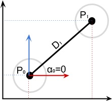
This means that, simply:
![\[P_1 = P_0 + D_1\]](https://www.alanzucconi.com/wp-content/ql-cache/quicklatex.com-c889c96e2dc93395f220405926d5903f_l3.png "Rendered by QuickLaTeX.com")
When is not zero, what we have to do is rotate the distance vector at rest  around by degrees:
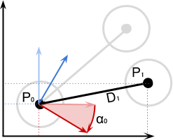
Mathematically we can write this as:
![\[P_1 = P_0 + rotate\left(D_1, P_0, \alpha_0\right)\]](https://www.alanzucconi.com/wp-content/ql-cache/quicklatex.com-f96e356f85df7fc94f6e3ca1136867fc_l3.png "Rendered by QuickLaTeX.com")
We will see later how we can use the function AngleAxis (Unity Documentation), without messing up with trigonometry.
By replicating the same logic, we can derive the equation for :
![\[P_2 = P_1 + rotate\left(D_2, P_1, \alpha_0 + \alpha_1\right)\]](https://www.alanzucconi.com/wp-content/ql-cache/quicklatex.com-0653ac1911d9ff07943698f03312fc49_l3.png "Rendered by QuickLaTeX.com")
And finally, the general equation:
![\[P_{i} = P_{i-1} + rotate\left(D_i, P_{i-1}, \sum_{k=0}^{i-1}\alpha_k\right)\]](https://www.alanzucconi.com/wp-content/ql-cache/quicklatex.com-7aa6ae4e17c0600f1f9f53ff2e6b3a5a_l3.png "Rendered by QuickLaTeX.com")
We will see in the next part of this tutorial, Implementing Forward Kinematics, how that equation will translated nicely to C# code.
❓ Forward Kinematics in 2D
![\[P_1^x = P_0^x + D_1^x \cos \alpha_0\]](https://www.alanzucconi.com/wp-content/ql-cache/quicklatex.com-cd46aacab8cbefef3a0c40ea13878993_l3.png "Rendered by QuickLaTeX.com")
![\[P_1^y = P_0^y + D_1^y \sin \alpha_0\]](https://www.alanzucconi.com/wp-content/ql-cache/quicklatex.com-296c88d5ba50192f941edcefbcc10297_l3.png "Rendered by QuickLaTeX.com")
For more information on the derivation, you can read A Gentle Primer on 2D Rotations.
❓ What about the Denavit-Hartenberg matrix?
This tutorial, however, will not rely on them. Solving a Denavit-Hartenberg matrix requires more Mathematics than most programmers are willing to do. The approach chosen relies on gradient descent, which is a more general optimisation algorithm.
Other Resources
- Part 1. An Introduction to Procedural Animations
- Part 2. The Mathematics of Forward Kinematics
- Part 3. Implementing Forward Kinematics
- Part 4. An Introduction to Gradient Descent
- Part 5. Inverse Kinematics for Robotic Arms
- Part 6. Inverse Kinematics for Tentacles
- Part 7. Inverse Kinematics for Spider Legs 🚧 (work in progress!)
Become a Patron!
Patreon You can download the Unity project for this tutorial on Patreon.
Credits for the 3D model of the robotic arm goes to Petr P.
💖 Support this blog
This website exists thanks to the contribution of patrons on Patreon. If you think these posts have either helped or inspired you, please consider supporting this blog.
📧 Stay updated
You will be notified when a new tutorial is released!
📝 Licensing
You are free to use, adapt and build upon this tutorial for your own projects (even commercially) as long as you credit me.
You are not allowed to redistribute the content of this tutorial on other platforms, especially the parts that are only available on Patreon.
If the knowledge you have gained had a significant impact on your project, a mention in the credit would be very appreciated. ❤️🧔🏻
Do you know how both approaches (Gradient Descent and Denavit-Hartenberg matrix) compare in terms of potential performance?
Hey!
It really depends on how they are implemented, and if the engine you are using has fast support for matrix multiplications and quaternions.
For me, the biggest advantage of using gradient descent is that you can specify arbitrary functions and conditions to minimise. Is not just about “reaching the target optimally”. It can be “reach the target but avoid touching this point”, or other stuff that you won’t be able to achieve with DH matrices!
In the third graphic under “Geometrical Interpretation”, you show the original rotations of P0 and P2 (pointing straight up), but for P1 you show it’s rotation from the previous graphic instead, failing to show that it is affected by angle0 and angle1.
It should either show only the local rotation changes (angle0 on P0, angle1 on P1, nothing on P2), or it should show the world rotation changes (angle0 on P0, angle0 and angle1 on P1, and angle0 and angle1 on P2), not half and half.
It appears to me that you don’t set Joints, SamplingDistance and DistanceThreshold. Or did I miss something? 🙂
Hey! You mean in the project or in the code shown in this tutorial?
Hi! In the tutorial! I havn’t downloaded the project 🙂
Yes, they have to be initialised in the Inspector!
PS: Thanks for an amazing tutorial!
Thanks for this awesome tutorial! For me the StartOffset don’t worked (the final position was never on the correct place)… what I did was calculating the distance between current and previous joint, and applyed it to the nextPoint vector:
float distanceFromLastJoint = Vector3.Distance(currentJoint.transform.position, lastJoint.transform.position);
rotation *= Quaternion.AngleAxis(lastJoint.angle, lastJoint.axis);
Vector3 nextPoint = prevPoint + rotation * (new Vector3(0, distanceFromLastJoint, 0));